2.2 - Electric Potential

Electric Potential vs. Electric Potential Energy

Electric potential energy describes the energy stored in a configuration of charges. Electric potential describes something different, and more fundamental.

Electric potential ( $V$ ): the electric potential energy per unit charge at a point in space.

V = \frac{U_e}{q}

The key distinction: - Electric potential energy ( $U$ ) depends on the system of charges, and is measured in joules. - Electric potential ( $V$ ) is a property of a point in space, independent of any test charge, and is measured in J/C or volts.

Think of it this way: electric potential describes the “energy landscape” that exists at every point in space, whether or not there’s a charge sitting there.

Example: Potential from Potential Energy

Problem: A

+4.0

nC test charge placed at point P has an electric potential energy of

2.4 \times 10^{-6}

J (with

U = 0

at infinity). (a) What is the electric potential at P? (b) The test charge is swapped for a

-2.0

nC charge. What is the potential at P now, and what is the new charge’s potential energy?

Solution (a):

V = \frac{U_E}{q} = \frac{2.4 \times 10^{-6} \text{ J}}{4.0 \times 10^{-9} \text{ C}} = 6.0 \times 10^2 \text{ V}

Solution (b): The potential is still

6.0 \times 10^2

V. It’s set by the charges that make the field, not by whatever test charge you put there. The potential energy does change:

U_E = qV = (-2.0 \times 10^{-9} \text{ C})(6.0 \times 10^2 \text{ V}) = -1.2 \times 10^{-6} \text{ J}

Answer: (a) 600 V. (b) Still 600 V, but now

U_E = -1.2 \times 10^{-6}

Electric Potential from Charge Distributions

For continuous charge distributions, potential requires integration using the principle of superposition.

The General Integration Formula

V = \frac{1}{4\pi\epsilon_0}\int \frac{dq}{r}

or equivalently:

V = k\int \frac{dq}{r}

where: -

V

= electric potential (V) -

k = 9 \times 10^9

N·m²/C² -

dq

= an infinitesimal charge element -

r

= distance from

dq

to the point

Important: notice that potential is a scalar, not a vector. There’s no

\hat{r}

unit vector like there was in the field integral. That often makes potential calculations a lot easier than field calculations.

Which Distributions Need Calculus

On the AP exam, you’ll only be asked to use calculus to find the potential in these cases: - An infinitely long, uniformly charged wire or cylinder, at some distance from its axis (done by integrating the field, in the Potential from Field section below). - A thin ring of charge, at a point on its axis. - A semicircular arc, or part of one, at its center. - A finite line of charge, at a point on the line itself or on its perpendicular bisector.

The Recipe

Pick a small piece of charge $dq$ and write it in terms of a length: $dq = \lambda\,dx$ for a straight line, or $dq = \lambda R\,d\theta$ for an arc, where $\lambda$ is the charge per length.

Write the distance $r$ from that piece to the point P, in terms of your variable.

Set up $V = k\int \frac{dq}{r}$ with limits that cover the whole object, then integrate.

Check a limit. Far away, every one of these should turn into $V \approx \frac{kQ}{d}$ , like a point charge.

Since

V

is a scalar, there’s no splitting into components and no canceling by symmetry like there was for the field. You just add up

\frac{k\,dq}{r}

Thin Ring, on Its Axis

Every piece of the ring is the same distance from P:

r = \sqrt{R^2 + x^2}

. So

r

comes out of the integral:

V = k\int \frac{dq}{\sqrt{R^2 + x^2}} = \frac{k}{\sqrt{R^2 + x^2}}\int dq = \frac{kQ}{\sqrt{R^2 + x^2}}

Checks: at the center (

x = 0

V = \frac{kQ}{R}

, even though the field there is zero. Far away (

x \gg R

V \approx \frac{kQ}{x}

, a point charge.

Example: A ring of radius 0.10 m carries

+5.0

nC spread evenly. Find the potential on its axis 0.24 m from the center.

V = \frac{(9.0 \times 10^9)(5.0 \times 10^{-9})}{\sqrt{(0.10)^2 + (0.24)^2}} = \frac{45 \text{ V}\cdot\text{m}}{0.26 \text{ m}} = 1.7 \times 10^2 \text{ V}

At the center it would be

\frac{(9.0 \times 10^9)(5.0 \times 10^{-9})}{0.10} = 4.5 \times 10^2

Semicircular Arc, at Its Center

Every piece of the arc is a distance

R

from the center, so

r

is constant again. With

dq = \lambda R\,d\theta

V = k\int_0^{\pi} \frac{\lambda R\,d\theta}{R} = k\lambda\pi = \frac{kQ}{R}

using

Q = \lambda\pi R

for a semicircle. For part of an arc that spans an angle

\theta_0

(in radians), the same steps give

V = k\lambda\theta_0

, which is still

\frac{kQ}{R}

with

Q

the charge on that piece. Compare that to the field at the center, which needs components and a

\sin\theta

integral. The potential doesn’t care about direction.

Example: A thin semicircular rod of radius 0.15 m carries

-6.0

nC spread evenly. Find the potential at its center. Then find it for a quarter-circle rod with the same radius and the same charge per length.

V_{semi} = \frac{kQ}{R} = \frac{(9.0 \times 10^9)(-6.0 \times 10^{-9})}{0.15} = -3.6 \times 10^2 \text{ V}

The quarter circle is half the arc, so it has half the charge (

-3.0

nC) at the same distance:

V_{quarter} = -1.8 \times 10^2

Finite Line of Charge, at a Point on the Line

Put the rod (length

L

, charge per length

\lambda

) from

x = 0

x = L

, with P a distance

d

past the right end. A piece at position

x

r = L + d - x

from P:

V = k\int_0^L \frac{\lambda\,dx}{L + d - x} = k\lambda\left[-\ln(L + d - x)\right]_0^L = k\lambda\ln\left(\frac{L + d}{d}\right)

Example: A 0.40 m rod carries

+8.0

nC spread evenly. Find the potential on its axis 0.10 m past one end.

\lambda = \frac{8.0 \times 10^{-9} \text{ C}}{0.40 \text{ m}} = 2.0 \times 10^{-8} \text{ C/m}, \quad k\lambda = (9.0 \times 10^9)(2.0 \times 10^{-8}) = 180 \text{ V}

V = (180 \text{ V})\ln\left(\frac{0.40 + 0.10}{0.10}\right) = (180 \text{ V})(\ln 5) = 2.9 \times 10^2 \text{ V}

Far away (

d \gg L

\ln\left(1 + \frac{L}{d}\right) \approx \frac{L}{d}

, so

V \approx \frac{k\lambda L}{d} = \frac{kQ}{d}

, a point charge again.

Finite Line of Charge, on Its Perpendicular Bisector

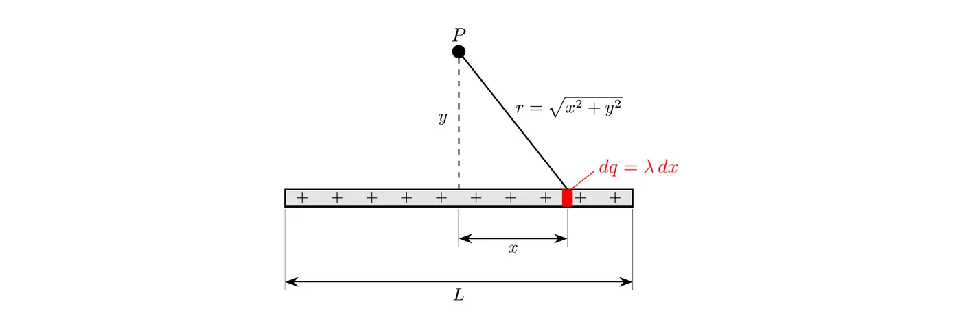
Center the rod on the origin so it runs from

x = -\frac{L}{2}

x = \frac{L}{2}

, with P a distance

y

above the middle. A piece at

x

r = \sqrt{x^2 + y^2}

from P. Using the standard integral

\int \frac{dx}{\sqrt{x^2 + y^2}} = \ln\left(x + \sqrt{x^2 + y^2}\right)

V = k\lambda\int_{-L/2}^{L/2} \frac{dx}{\sqrt{x^2 + y^2}} = k\lambda\ln\left(\frac{\frac{L}{2} + \sqrt{\frac{L^2}{4} + y^2}}{-\frac{L}{2} + \sqrt{\frac{L^2}{4} + y^2}}\right)

Example: Same rod as above (0.40 m long,

k\lambda = 180

V). Find the potential 0.15 m from its midpoint, on the perpendicular bisector. Here

\frac{L}{2} = 0.20

m and

\sqrt{(0.20)^2 + (0.15)^2} = 0.25

V = (180 \text{ V})\ln\left(\frac{0.20 + 0.25}{-0.20 + 0.25}\right) = (180 \text{ V})(\ln 9) = 4.0 \times 10^2 \text{ V}

Electric Potential from Point Charges

A Single Point Charge

For a single point charge, the potential at distance

r

is:

V = k\frac{Q}{r}

where: -

V

= electric potential (V, or J/C) -

Q

= source charge (C) -

r

= distance from the charge (m)

Key features: - Potential is a scalar, so it has no direction. - The sign follows the sign of

Q

: a positive charge gives

V > 0

, and a negative charge gives

V < 0

. -

V \to 0

r \to \infty

, which is the reference point.

Example: Find the potential 0.30 m from a

-6.0

nC point charge, and the distance where the potential is half that.

V = k\frac{Q}{r} = (9.0 \times 10^9)\frac{-6.0 \times 10^{-9}}{0.30} = -1.8 \times 10^2 \text{ V}

Since

V \propto \frac{1}{r}

, half the potential (

-90

V) is at twice the distance, 0.60 m. Compare the field, which goes as

\frac{1}{r^2}

: doubling the distance cuts

E

to a quarter (from

6.0 \times 10^2

N/C to

1.5 \times 10^2

N/C).

Multiple Point Charges

For a system of point charges, use superposition and just add the values algebraically:

V = k\sum_{i} \frac{Q_i}{r_i}

where

r_i

is the distance from charge

Q_i

to the point you care about.

The critical point: unlike forces and fields, you add potentials as scalars, not vectors. Just add the numbers, keeping their signs.

Zero potential doesn’t mean zero field, and zero field doesn’t mean zero potential. Potential adds as a scalar and the field adds as a vector, so they can behave very differently at the same point. Take two charges 0.20 m apart and look at the midpoint, 0.10 m from each: - Opposite charges (

+3.0

nC and

-3.0

nC): the potentials cancel, so

V = 0

. But both fields point toward the negative charge, so they add:

E = 2k\frac{q}{r^2} = 2(9.0 \times 10^9)\frac{3.0 \times 10^{-9}}{(0.10)^2} = 5.4 \times 10^3

N/C. - Like charges (two

+3.0

nC charges): the fields point opposite ways and cancel, so

E = 0

. But the potentials add:

V = 2k\frac{q}{r} = 2(9.0 \times 10^9)\frac{3.0 \times 10^{-9}}{0.10} = 5.4 \times 10^2

Electric Potential Difference

The potential difference between two points is the change in potential energy per unit charge when you move a test charge between them.

\Delta V = V_B - V_A = \frac{\Delta U_e}{q}

What it means physically: the potential difference tells you how much work per unit charge it takes to move a charge from point A to point B.

Units: volts (V) = joules per coulomb (J/C).

1 \text{ V} = 1 \text{ J/C}

Example: Potential Difference from Work

Problem: As a

+3.0

μC charge moves from point A to point B, the electric field does

+6.0 \times 10^{-4}

J of work on it. (a) Find the change in electric potential energy. (b) Find

V_B - V_A

. (c) An electron moves from A to B instead. What is its change in potential energy?

(a) The work done by the field is the negative of the change in potential energy:

\Delta U_E = -W_{field} = -6.0 \times 10^{-4} \text{ J}

(b) Divide by the charge:

\Delta V = V_B - V_A = \frac{\Delta U_E}{q} = \frac{-6.0 \times 10^{-4} \text{ J}}{3.0 \times 10^{-6} \text{ C}} = -2.0 \times 10^2 \text{ V}

(c) The potential difference between A and B doesn’t depend on what moves, so it’s still

-2.0 \times 10^2

\Delta U_E = q\Delta V = (-1.60 \times 10^{-19} \text{ C})(-2.0 \times 10^2 \text{ V}) = +3.2 \times 10^{-17} \text{ J}

Answer: B is 200 V lower than A. The positive charge loses potential energy going there, while the electron gains it.

Potential Difference from Chemical Processes: Batteries

A potential difference doesn’t have to come from charges you placed somewhere. In a battery, chemical reactions separate charge: they pull electrons off one electrode and pile them onto the other. That leaves the positive terminal short on electrons (higher potential) and the negative terminal with extra electrons (lower potential), so there’s a potential difference between them.

To keep that separation going, the chemical reactions do work on the charges, pushing them “uphill” against the electric force inside the battery. That energy comes from the chemical energy stored in the battery. A battery with a potential difference

\Delta V

between its terminals gives every coulomb it moves

\Delta V

joules of electric potential energy:

\Delta U_E = q\Delta V

So a 1.5 V battery gives each coulomb 1.5 J. The voltage is set by the battery’s chemistry, not its size. Circuits, EMF, and internal resistance come back in Unit 4.

Example: A 9.0 V battery moves 0.40 C of positive charge from its negative terminal to its positive terminal (in a real battery it’s electrons moving the other way, which has the same effect). How much chemical energy turns into electric potential energy?

\Delta U_E = q\Delta V = (0.40 \text{ C})(9.0 \text{ V}) = 3.6 \text{ J}

The Relationship Between Field and Potential

Electric field and electric potential are tightly connected through calculus.

Field from Potential (Differentiate)

The field component in any direction is the negative rate of change of potential:

E_x = -\frac{dV}{dx}

More generally, in vector form:

\vec{E} = -\nabla V = -\left(\frac{\partial V}{\partial x}\hat{x} + \frac{\partial V}{\partial y}\hat{y} + \frac{\partial V}{\partial z}\hat{z}\right)

The key principle: the electric field points in the direction of decreasing potential, which is where the negative sign comes from.

Reading the Field from a V vs. x Graph

Since

E_x = -\frac{dV}{dx}

, the field is the negative slope of a

V

vs.

x

graph: - Where

V

goes up as

x

increases,

E_x

is negative (the field points toward

-x

). - Where

V

is flat,

E_x = 0

. - Where

V

goes down,

E_x

is positive. - A steeper slope means a stronger field.

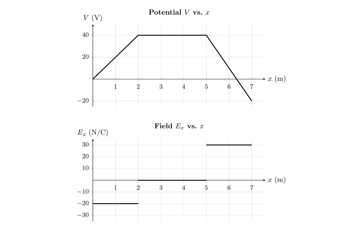
In these graphs: - From

x = 0

to 2 m,

V

rises 40 V over 2 m, a slope of

+20

V/m, so

E_x = -20

N/C. - From 2 m to 5 m,

V

stays at 40 V, so

E_x = 0

. A charge there feels no electric force. - From 5 m to 7 m,

V

drops 60 V over 2 m, a slope of

-30

V/m, so

E_x = +30

N/C.

(1 V/m is the same as 1 N/C.) To predict motion, remember that a positive charge is pushed toward lower

V

and a negative charge toward higher

V

. A proton at

x = 6

m is pushed toward

+x

. An electron at

x = 1

m is pushed toward

+x

too, uphill in

V

toward the 40 V plateau.

Example: Field from a Potential Function

Problem: Along the x-axis, the potential is

V(x) = 40x^2 - 160x + 200

, with

V

in volts and

x

in meters. (a) Find

E_x

x = 0.50

m and at

x = 3.0

m. (b) Where is the field zero? (c) Find the force on an electron at

x = 0.50

(a) Take the derivative and flip the sign:

E_x = -\frac{dV}{dx} = -(80x - 160) = 160 - 80x

E_x(0.50) = 160 - 80(0.50) = 1.2 \times 10^2 \text{ N/C}, \quad E_x(3.0) = 160 - 80(3.0) = -80 \text{ N/C}

At 0.50 m the field points toward

+x

. At 3.0 m it points toward

-x

(b)

E_x = 0

when

160 - 80x = 0

, so

x = 2.0

m. That’s the bottom of the

V

curve, where the slope is zero.

(c)

F_x = qE_x = (-1.60 \times 10^{-19} \text{ C})(1.2 \times 10^2 \text{ N/C}) = -1.9 \times 10^{-17}

N. The force on the electron points toward

-x

, toward higher potential.

Potential from Field (Integrate)

Going the other way, you find the potential difference by integrating the field:

\Delta V = V_B - V_A = -\int_A^B \vec{E} \cdot d\vec{r}

Or, in terms of the angle between the field and the path:

\Delta V = -\int_A^B E \cos\theta \, dr

That negative sign means moving with the field decreases the potential.

For a uniform field,

E

comes out of the integral, and what’s left is just the part of the displacement along the field:

\Delta V = -\vec{E} \cdot \Delta\vec{r} = -Ed\cos\theta

where

d

is the distance from A to B and

\theta

is the angle between

\vec{E}

and the displacement. Moving perpendicular to the field (

\theta = 90^\circ

) doesn’t change

V

at all.

Example: Potential Difference in a Uniform Field

Problem: A uniform 500 N/C field points in the

+x

direction. Point B is 0.40 m to the right of point A and 0.30 m above it. Find

V_B - V_A

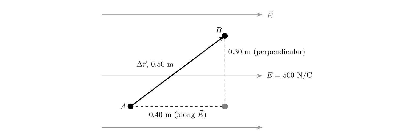
Only the 0.40 m along the field matters. Using the full displacement gives the same thing:

d = 0.50

m and

\cos\theta = \frac{0.40}{0.50}

\Delta V = -Ed\cos\theta = -(500 \text{ N/C})(0.50 \text{ m})\left(\frac{0.40}{0.50}\right) = -2.0 \times 10^2 \text{ V}

Answer: B is 200 V lower than A. The 0.30 m sideways part of the trip changes nothing, and since the electric force is conservative, any path from A to B gives the same answer.

Infinitely Long Line or Cylinder of Charge

For an infinite line of charge, you can’t use

V = k\int\frac{dq}{r}

with

V = 0

at infinity: there’s an infinite amount of charge, and the integral blows up. Instead, find the difference in potential by integrating the field. Topic 1.6 (Cylindrical Symmetry) used Gauss’s law with a cylindrical surface to find the field a distance

r

from a line (or outside a uniformly charged cylinder) with charge per length

\lambda

E = \frac{\lambda}{2\pi\epsilon_0 r} = \frac{2k\lambda}{r}

pointing straight out from the axis (for

\lambda > 0

). Integrating outward from

r_a

r_b

\Delta V = V_b - V_a = -\int_{r_a}^{r_b} \frac{2k\lambda}{r}\,dr = -2k\lambda\ln\left(\frac{r_b}{r_a}\right)

Since

\ln r

keeps growing as

r \to \infty

, there’s no way to set

V = 0

at infinity. Problems either ask for a difference or pick a zero at some finite distance.

Example: A long, thin wire carries

\lambda = +4.0

nC/m. Find

V_b - V_a

between

r_a = 2.0

cm and

r_b = 8.0

cm from the wire.

\Delta V = -2(9.0 \times 10^9)(4.0 \times 10^{-9})\ln\left(\frac{8.0}{2.0}\right) = -(72 \text{ V})(\ln 4) = -1.0 \times 10^2 \text{ V}

The point closer to the wire is about 100 V higher, which makes sense: the field points away from a positive line, toward lower potential.

Inside a uniformly charged solid cylinder (radius

R

, charge per length

\lambda

), only the fraction

\frac{r^2}{R^2}

of the charge is enclosed, so Gauss’s law gives

E = \frac{2k\lambda r}{R^2}

(the same as 1.6’s

\frac{\rho r}{2\epsilon_0}

, with

\lambda = \rho\pi R^2

). Then the axis is higher than the surface by

V(0) - V(R) = \int_0^R \frac{2k\lambda r}{R^2}\,dr = k\lambda

Potential Graphs: Conductors vs. Insulators

Electric potential behaves very differently in conductors versus insulators at electrostatic equilibrium.

Conductor

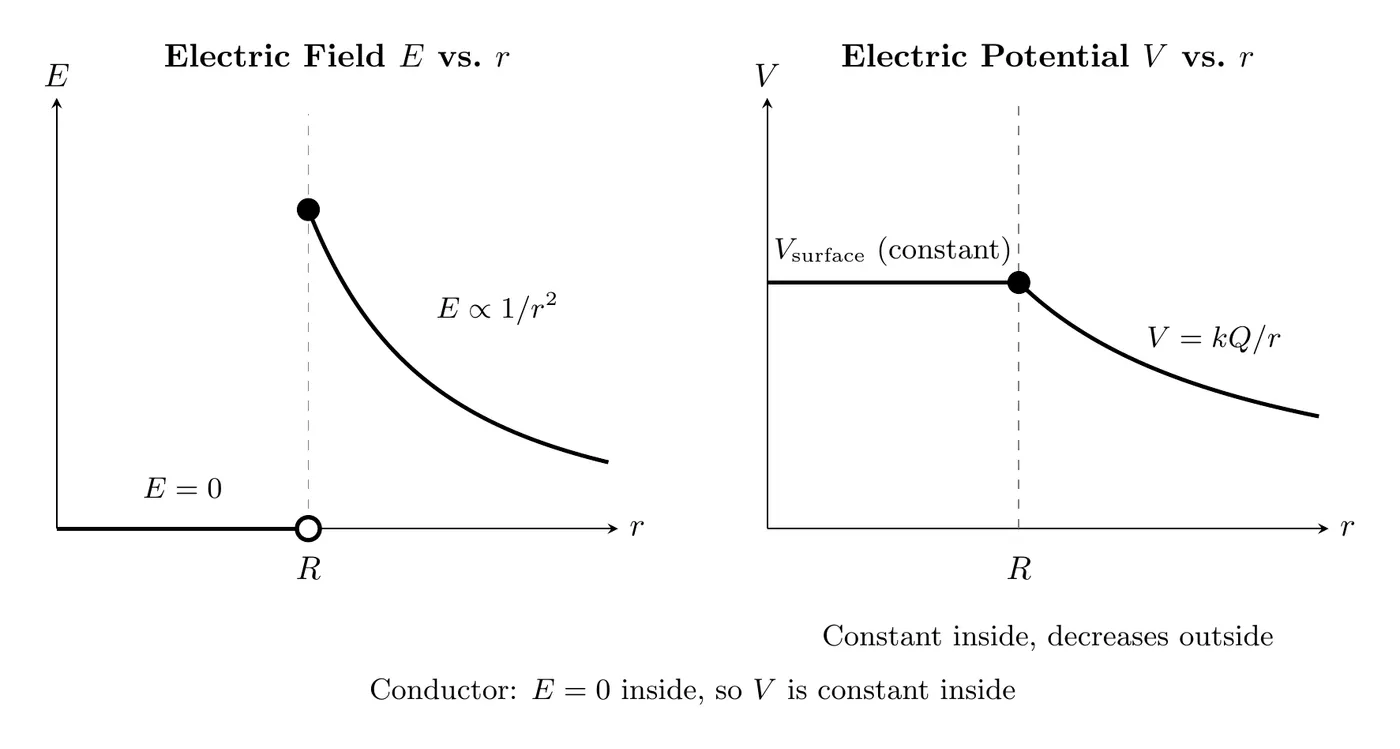
Key features: - Inside the conductor:

E = 0

, so

V = \text{constant}

. - At the surface:

V

is continuous, with no jump. - Outside:

V = \frac{kQ}{r}

, the same as a point charge.

Why is it constant inside? Since

E = -\frac{dV}{dr}

, if

E = 0

, then

\frac{dV}{dr} = 0

, which means

V

doesn’t change.

Insulator

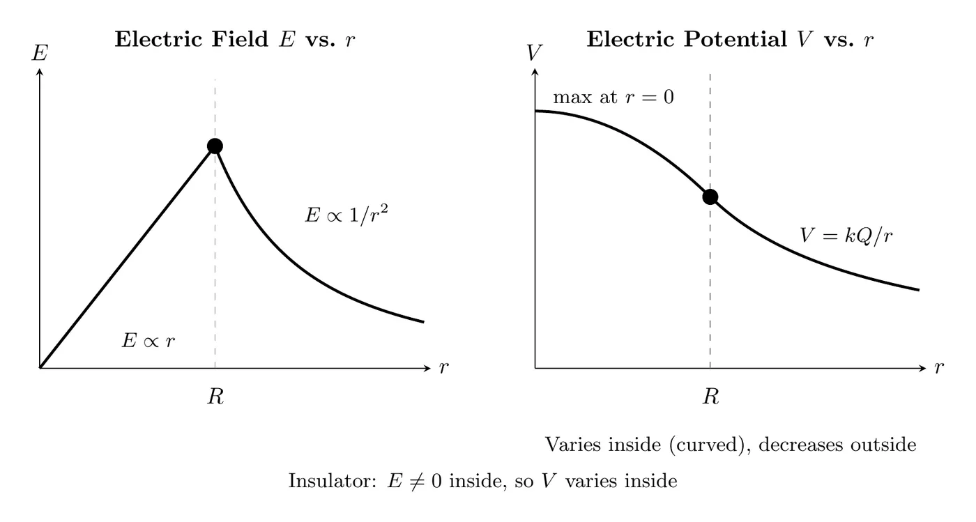
Key features: - Inside the insulator:

E \neq 0

, so

V

varies and the graph is curved. - At the center:

V

is at its maximum. - Outside:

V = \frac{kQ}{r}

, the same as a point charge.

Equipotential Lines and Surfaces

Equipotential lines (in 2D) or equipotential surfaces (in 3D) are the places where the electric potential has the same value.

Properties

The electric field is perpendicular to the equipotential lines and surfaces everywhere.

It takes no work to move a charge along an equipotential, since $\Delta V = 0$ .

Closer spacing means a stronger field, because the potential is changing more steeply.

The field points toward decreasing potential, so from high $V$ to low $V$ .

There’s no field component along an equipotential line.

A Single Point Charge

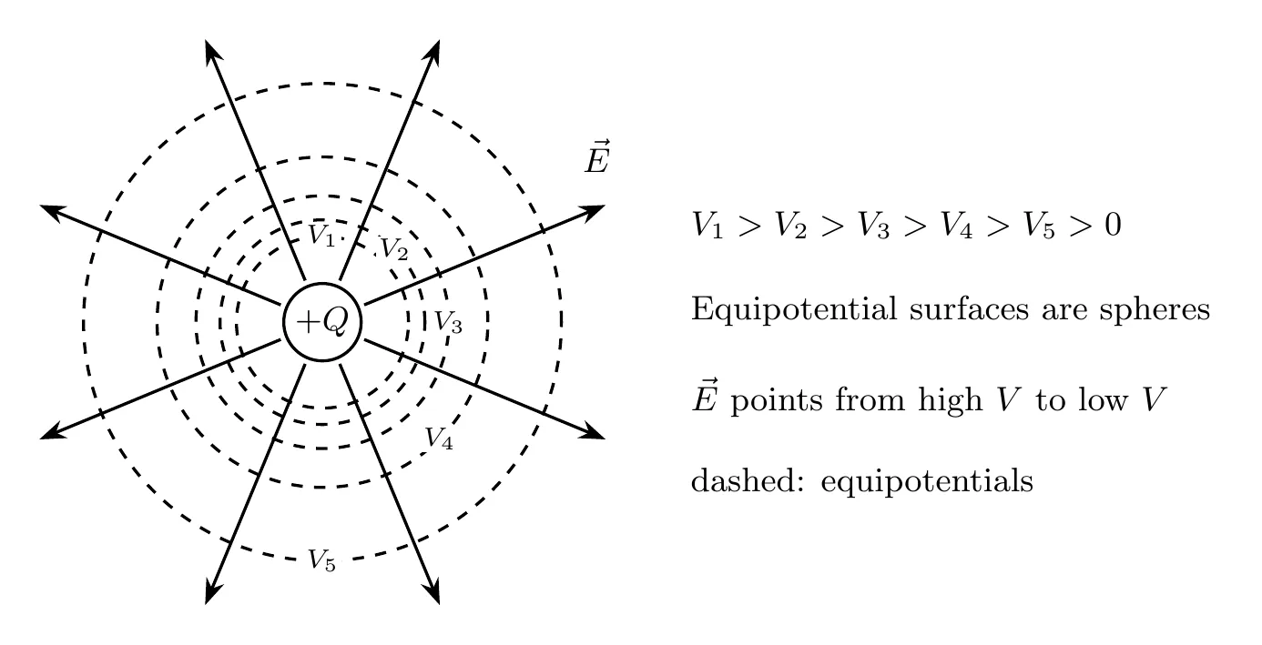
For a negative charge, the pattern looks the same, but the potential values are negative and the field points inward.

Multiple Charges (a Dipole)

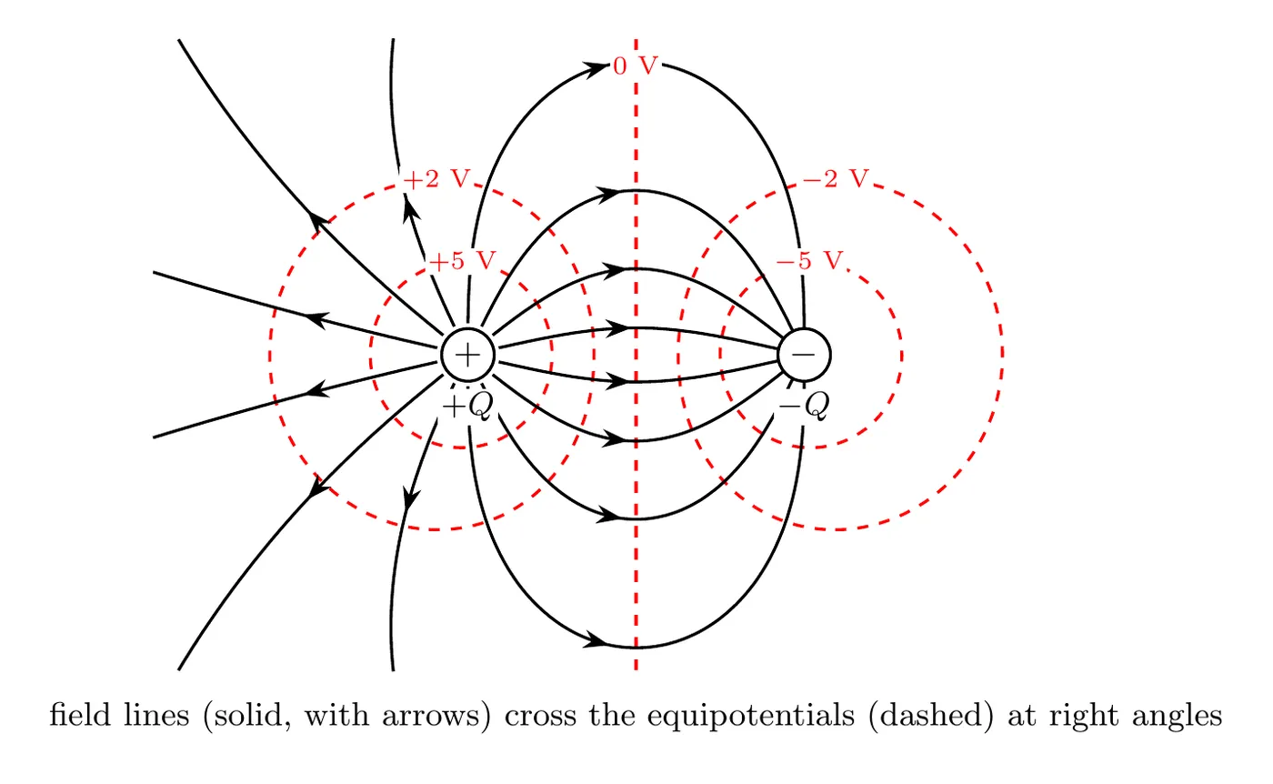
A useful analogy: equipotential lines work like the contour lines on a topographic map. - Contour lines show constant elevation, while equipotentials show constant potential. - Close spacing means steep terrain, which means a strong field. - Wide spacing means gentle terrain, which means a weak field.

Isolines and Field Maps

Equipotential lines are also called isolines of electric potential (“iso” means equal). A field vector map and an isoline map show the same field in two ways, and you can build either one from the other: - From a field map to isolines: draw curves that cross every field vector at a right angle. - From isolines to a field map: draw vectors perpendicular to the isolines, pointing from higher

V

toward lower

V

. Make them longer where the isolines are closer together. - Estimating the field strength: between two neighboring isolines,

E \approx \frac{|\Delta V|}{\Delta s}

, where

\Delta s

is the perpendicular distance between them. - Nothing along an isoline: the field has no component along an isoline, so moving along one takes no work.

Predicting motion: a positive charge released from rest accelerates along

\vec{E}

, toward lower potential. A negative charge accelerates opposite to

\vec{E}

, toward higher potential. Either way, the force starts out perpendicular to the isoline the charge is sitting on.

Example: Reading an Isoline Map

Problem: The map shows isolines in a region of space, with their values in volts. (a) Which way does the field point at P? (b) Estimate the field strength at P. (c) How much work does the field do on a

+2.0

nC charge that moves from A to B? (d) How much work does it do on a charge that moves from C to D? (e) Which way does an electron released from rest at P start to move?

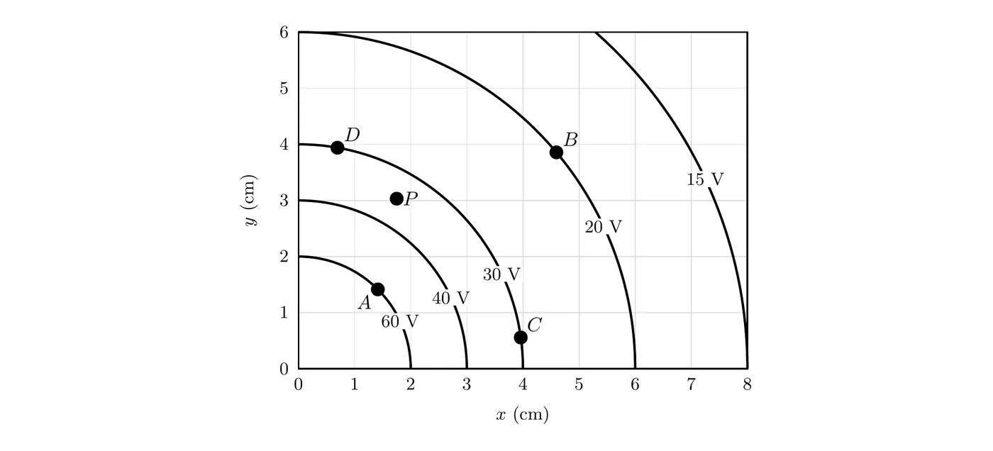
(a) Perpendicular to the isolines, toward lower

V

. At P that’s away from the lower-left corner (up and to the right), from the 40 V line toward the 30 V line.

(b) Near P, the 40 V and 30 V lines are about 1.0 cm apart:

E \approx \frac{|\Delta V|}{\Delta s} = \frac{10 \text{ V}}{0.010 \text{ m}} = 1.0 \times 10^3 \text{ V/m}

(c) A is on the 60 V line and B is on the 20 V line, so

\Delta V = 20 \text{ V} - 60 \text{ V} = -40

W_{field} = -q\Delta V = -(2.0 \times 10^{-9} \text{ C})(-40 \text{ V}) = +8.0 \times 10^{-8} \text{ J}

(d) C and D are both on the 30 V line, so

\Delta V = 0

and the field does no net work, whatever path the charge takes between them.

(e) Toward higher potential, opposite the field: down and to the left, toward the 40 V line.

(These isolines are circles centered on the lower-left corner, the pattern of a positive point charge sitting there with

kQ = 1.2

V·m:

\frac{1.2}{0.020} = 60

\frac{1.2}{0.030} = 40

V, and so on. Its exact field at P, 3.5 cm from the corner, is

\frac{kQ}{r^2} = \frac{1.2}{(0.035)^2} \approx 9.8 \times 10^2

V/m, close to the estimate.)

Example Problem 1: Potential from Multiple Charges

Problem: Three point charges sit at the vertices of an equilateral triangle with side length

a = 2.0

q_1 = +3.0

μC (top),

q_2 = -4.0

μC (bottom left), and

q_3 = +5.0

μC (bottom right). Find the electric potential at the center of the triangle.

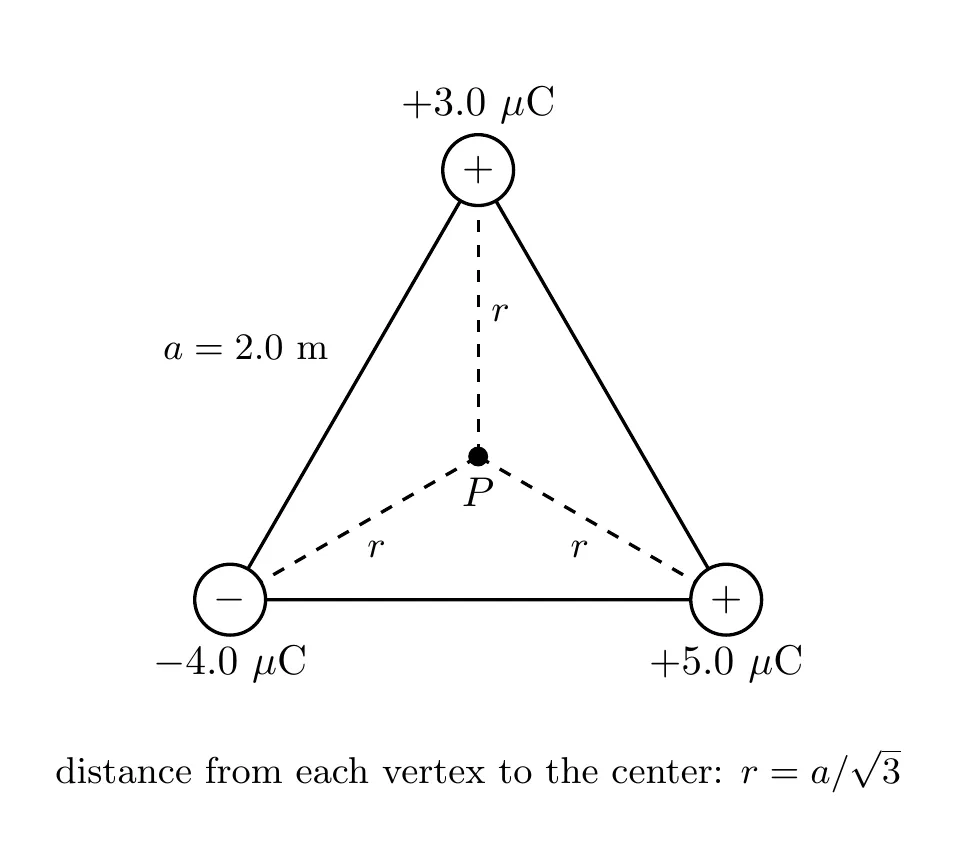
Solution

Step 1: Find the distance from each charge to the center

For an equilateral triangle with side

a

, the distance from any vertex to the center is:

r = \frac{a}{\sqrt{3}} = \frac{2.0}{\sqrt{3}} = 1.155 \text{ m}

Step 2: Apply superposition

V_{total} = V_1 + V_2 + V_3 = k\left(\frac{q_1}{r} + \frac{q_2}{r} + \frac{q_3}{r}\right)

Step 3: Factor and substitute

V_{total} = \frac{k}{r}(q_1 + q_2 + q_3)

Convert the charges to coulombs: -

q_1 = +3.0 \times 10^{-6}

C -

q_2 = -4.0 \times 10^{-6}

C -

q_3 = +5.0 \times 10^{-6}

V_{total} = \frac{9 \times 10^9}{1.155}(3.0 - 4.0 + 5.0) \times 10^{-6}

V_{total} = \frac{9 \times 10^9}{1.155}(4.0 \times 10^{-6})

V_{total} = 3.12 \times 10^4 \text{ V} = 31.2 \text{ kV}

Answer: the potential at the center is about 31.2 kV.

Example Problem 2: Potential Difference Between Two Points

Problem: A spherical conductor of radius

R

carries charge

+Q

. A concentric spherical shell of inner radius

4R

surrounds it. Derive an expression for the absolute value of the potential difference between the outer surface of the inner sphere (at

r = R

) and the inner surface of the shell (at

r = 4R

Given: the electric field in the region

R < r < 4R

E = \frac{Q}{4\pi\epsilon_0 r^2}

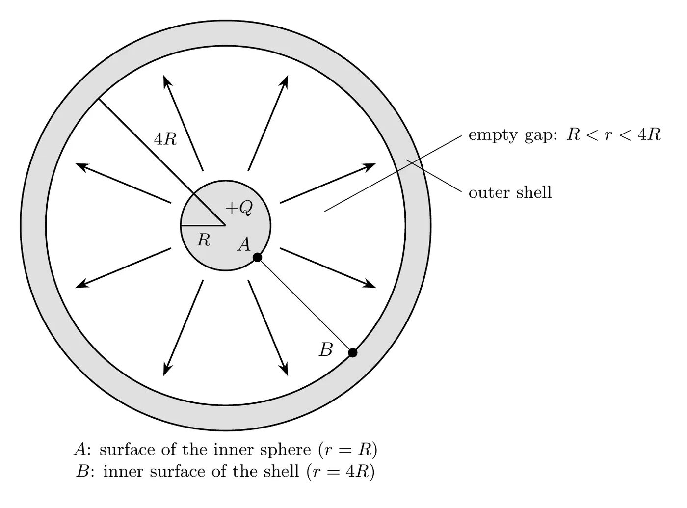
Solution

Step 1: Set up the potential difference integral

\Delta V = V_B - V_A = -\int_A^B \vec{E} \cdot d\vec{r}

Since

\vec{E}

points radially and we’re integrating radially:

\Delta V = -\int_R^{4R} E \, dr

Step 2: Substitute the given field

\Delta V = -\int_R^{4R} \frac{Q}{4\pi\epsilon_0 r^2} \, dr

Step 3: Factor out the constants

\Delta V = -\frac{Q}{4\pi\epsilon_0} \int_R^{4R} \frac{dr}{r^2}

Step 4: Rewrite for integration

\Delta V = -\frac{Q}{4\pi\epsilon_0} \int_R^{4R} r^{-2} \, dr

Step 5: Integrate with the power rule

\Delta V = -\frac{Q}{4\pi\epsilon_0} \left[\frac{r^{-1}}{-1}\right]_R^{4R}

\Delta V = -\frac{Q}{4\pi\epsilon_0} \left[-\frac{1}{r}\right]_R^{4R}

\Delta V = \frac{Q}{4\pi\epsilon_0} \left[\frac{1}{r}\right]_R^{4R}

Step 6: Evaluate the limits

\Delta V = \frac{Q}{4\pi\epsilon_0} \left(\frac{1}{4R} - \frac{1}{R}\right)

\Delta V = \frac{Q}{4\pi\epsilon_0} \left(\frac{1 - 4}{4R}\right)

\Delta V = \frac{Q}{4\pi\epsilon_0} \left(\frac{-3}{4R}\right)

\Delta V = -\frac{3Q}{16\pi\epsilon_0 R}

Step 7: Take the absolute value

|\Delta V| = \frac{3Q}{16\pi\epsilon_0 R}

Using

k = \frac{1}{4\pi\epsilon_0}

|\Delta V| = \frac{3kQ}{4R}

Answer: the magnitude of the potential difference is

\frac{3kQ}{4R}

, or equivalently

\frac{3Q}{16\pi\epsilon_0 R}

Key Relationships Summary

Quantity	From Field	From Potential
Potential	$V = -\int \vec{E} \cdot d\vec{r}$	Given
Field	Given	$\vec{E} = -\nabla V$ , or $E = -\frac{dV}{dr}$
Work	$W = \int \vec{F} \cdot d\vec{r}$	$W = q\Delta V$
PE change	$\Delta U = -W_{field}$	$\Delta U = q\Delta V$

Important Signs

$\vec{E}$ points from high to low potential.

Moving with the field: $\Delta V < 0$ , so the potential decreases.

Moving against the field: $\Delta V > 0$ , so the potential increases.

Work done by the field = $-q\Delta V$ .

Work done by an external force = $+q\Delta V$ .

Potential Inside vs. Outside Summary

Location	Conductor	Insulator (uniform)
Interior	$V = \text{constant}$	$V$ varies (parabolic)
Surface	Continuous	Continuous
Exterior	$V = \frac{kQ}{r}$	$V = \frac{kQ}{r}$

Common Mistakes

Treating potential as a vector. Potential is a scalar. Don’t try to add components or use vector addition. Just add the numbers with their signs.

Forgetting the negative sign in $E = -dV/dx$ . The field points toward decreasing potential, which is why the negative sign is there. Dropping it flips the direction.

Confusing V and U. Electric potential $V$ is measured in volts (J/C) and exists at a point. Potential energy $U$ is measured in joules and requires a charge. They’re linked by $U = qV$ .

Using the wrong limits in potential integrals. When you calculate $\Delta V = V_B - V_A$ , the integral is $-\int_A^B \vec{E} \cdot d\vec{r}$ . The order matters, and it affects the sign.

Assuming the potential is zero at a conductor’s surface. A conductor’s surface has constant potential, but that value isn’t necessarily zero. Zero potential is defined at infinity, or at ground if the problem specifies.

Back Next