

4.6 - Approximating Values of a Function Using Local Linearity and Linearization
The Big Idea
A tangent line to a function at a point can be used to approximate values of the function at points close to .
The closer you are to the point of tangency, the better the approximation. The farther away you go, the worse it gets.
Concavity and Estimation
Concave Up
A function is concave up when it curves upward like a cup (∪).
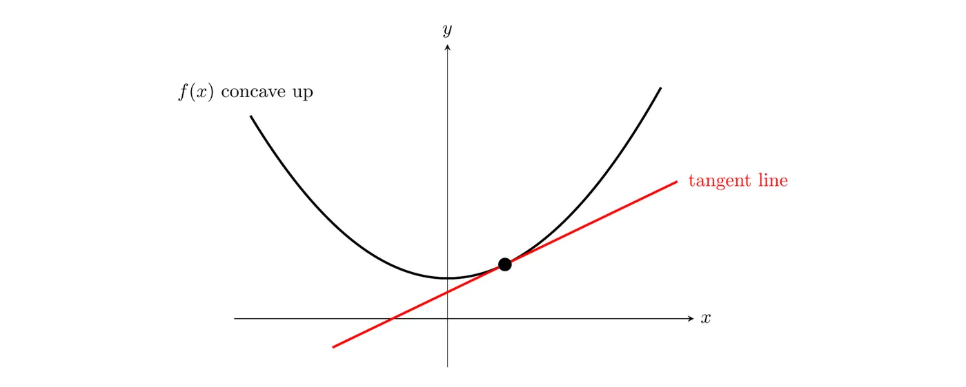
Key observation: when a function is concave up, the tangent line sits below the curve.
Concave Down
A function is concave down when it curves downward like a frown (∩).
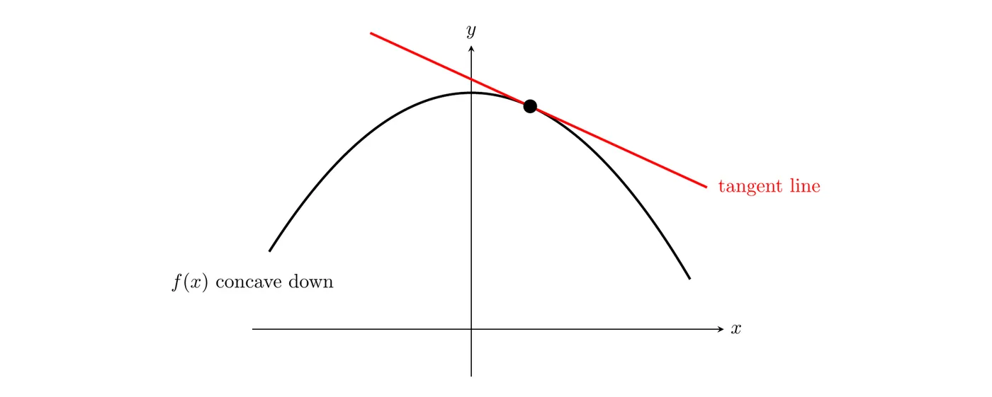
Key observation: when a function is concave down, the tangent line sits above the curve.
Local Linear Approximation
Definition: using a tangent line at to approximate function values near .
“Local” means we’re only looking at points close to . “Linear” means we’re using a line, the tangent line, to approximate the curve.
Why it works: when you zoom in very close to any smooth curve, it looks approximately like a straight line.
The Process
Step 1: Find the Tangent Line at
Use point-slope form:
You need the point and the slope .
Step 2: Use the Tangent Line to Approximate
To estimate where is close to , substitute into the tangent line equation:
That -value approximates .
Step 3: Determine Whether It’s an Over or Underestimate
- Concave up → underestimate
- Concave down → overestimate
If the problem doesn’t give the concavity, find it with the second derivative near : means concave up (underestimate), and means concave down (overestimate). From a graph of , the same idea works: increasing means concave up, and decreasing means concave down.
Example 1: Using Given Information
Given: is concave up on its domain, , and .
Find: an estimate for using local linear approximation.
Step 1: Write the tangent line at
Point , slope :
Alternative form, which is easier for substitution:
Step 2: Estimate
Answer:
Step 3: Determine the type of estimate
This is an underestimate because is concave up.
Justification to write: “This is an underestimate because is concave up.”
Example 2: With an Actual Function
Given: is concave down at .
Find: use the tangent line at to estimate .
Step 1: Find the point
So the point is .
Step 2: Find the slope
Step 3: Write the tangent line
Step 4: Estimate
Answer:
Step 5: Determine the type of estimate
This is an overestimate because is concave down at .
Justification to write: “This is an overestimate because is concave down.”
You can check the concavity yourself: , so , which confirms is concave down at .
Example 3: Differential Equation
Given: let be the particular solution to the differential equation
with the initial condition .
Find: write the equation of the tangent line at and use it to approximate .
Understanding the Setup
Differential equation: an equation involving derivatives. Here gives us the slope directly.
Particular solution: there’s some function that satisfies this differential equation.
Initial condition: we know the function passes through the point .
Solution
Step 1: Find the point
We’re given from the initial condition.
Step 2: Find the slope at
Use the differential equation with and :
Step 3: Write the tangent line
Expanded:
Step 4: Estimate
Answer:
Note: we can still decide whether this is an over or underestimate by finding the concavity from the differential equation. Differentiate again, using the product rule and the chain rule (since is a function of ):
At , where :
Since , is concave up near , so is an underestimate.
Linearization Formula
The general formula for linear approximation:
where:
- is the linearization (the tangent line) at
- is the function value at
- is the derivative, meaning the slope, at
To approximate :
Practice Problem
Given: , and we want to approximate using the tangent line at .
Find the point:
Find the slope:
Write the tangent line:
Estimate :
Therefore:
Type of estimate: since is concave down, this is an overestimate.
Why This Matters
Linear approximation is useful when:
- Calculations are difficult. Approximating without a calculator
- The function is unknown. You only have limited information about
- You need a quick estimate. Fast approximation without heavy computation
- You want to understand behavior. Seeing how functions act near a point
Common Mistakes
- ❌ Using the wrong form. Make sure you’re using point-slope form correctly
- ❌ Wrong sign on the slope. Be careful with negative slopes
- ❌ Concavity confusion. Concave up means underestimate, concave down means overestimate
- ❌ Approximating too far away. Linear approximation only works well near the tangent point
- ❌ Forgetting the justification. Always explain why it’s an over or underestimate using concavity
Key Takeaways
- Tangent lines approximate functions near the point of tangency
- Linearization formula:
- Concave up → underestimate, since the tangent line is below the curve
- Concave down → overestimate, since the tangent line is above the curve
- Closer is better. Approximations improve the closer you are to the tangent point
- Point-slope form is easier. is convenient for substitution
- Differential equations give you directly, which is the slope
- Always justify. State “underestimate/overestimate because concave up/down”
- No concavity given? Use the sign of near the point to decide
- Local linear approximation is just another name for using tangent lines to approximate
- Works for any smooth curve, since when you zoom in, curves look like lines