

3.2 - Redistribution of Charge between Conductors
Charge Redistribution in Connected Conductors
When two or more conductors are put into electrical contact (say, by hooking them together with a conducting wire), charge shuffles between them until everything settles into electrostatic equilibrium.
The Fundamental Principle: Equal Potential
Once conductors are connected, they become a single equipotential system. The defining feature is:
Every connected conductor ends up at the same electric potential.
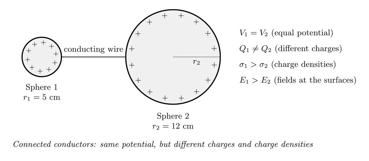
What Matches and What Doesn’t
When conductors are connected and sitting at equilibrium:
Equal between connected conductors
✓ Electric potential
NOT equal between connected conductors
✗ Total charge
✗ Surface charge density
✗ Electric field at the surface
✗ Surface area
Relationships for Spherical Conductors
For two connected conducting spheres with different radii, here’s how things shake out.
The Potential Relationship
They’re both at the same potential:
which simplifies to:
So charge is proportional to radius:
The bigger sphere ends up with more total charge. But charge density is a whole different story.
Surface Charge Density
Surface charge density is:
For a sphere, , so:
And since :
So surface charge density goes inversely with radius:
The key result: the smaller sphere has the higher surface charge density, even though it holds less total charge.
Electric Field at the Surface
Just outside a spherical conductor:
And since :
So the field also goes inversely with radius:
The key result: the smaller sphere has the stronger field at its surface.
Summary Table: Size vs. Properties
Property | Larger Sphere | Smaller Sphere |
Radius | Large | Small |
Potential | Same | Same |
Total charge | More | Less |
Surface area | More | Less |
Charge density | Less | More |
Surface field | Weaker | Stronger |
The inverse relationships:
- As the radius goes up, the charge density goes down.
- As the radius goes up, the surface field goes down.
Grounding
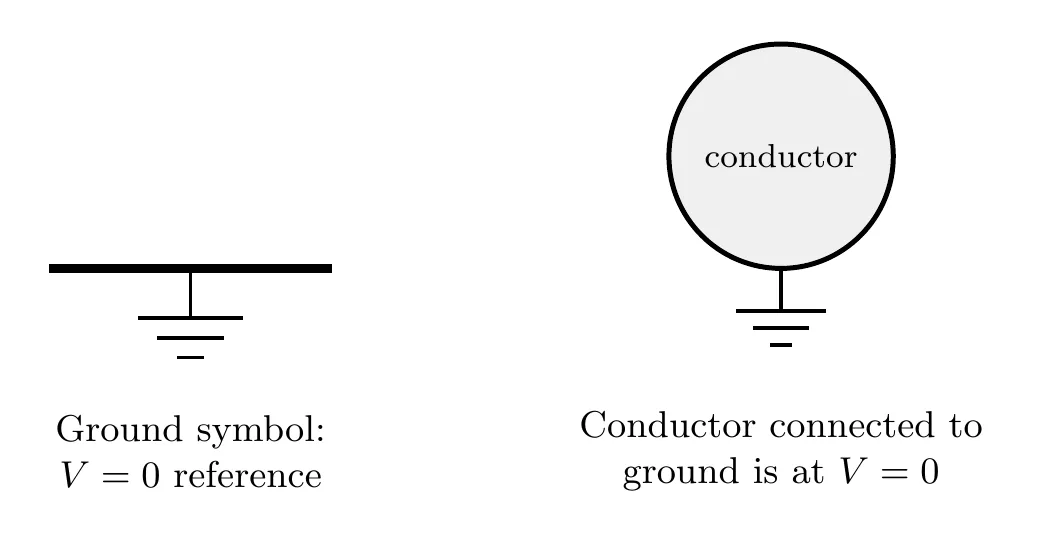
Grounding sets up an idealized reference point at zero electric potential.
What It Means
A grounded conductor:
- Has by definition.
- Can soak up or hand over an unlimited amount of charge.
- Stays at no matter how much charge moves through.
The Earth is the universal ground reference in most situations.
The Grounding Symbol
Where You Actually See It: Static Discharge Straps
If you’re working with sensitive electronics (building a computer, handling circuit boards):
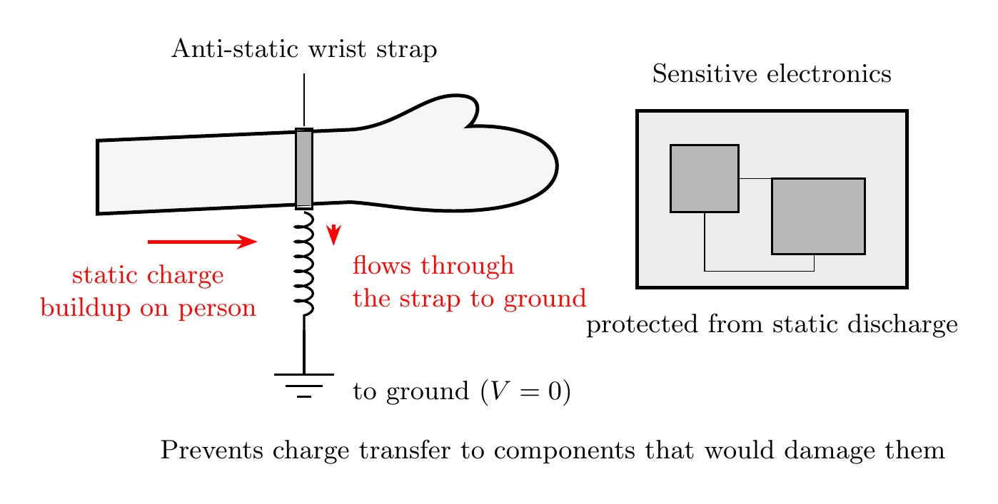
Why it matters:
- Static charge naturally piles up on your body.
- Without grounding, touching electronics dumps that charge into them.
- Even a small discharge can fry sensitive components, causing short circuits or burnt traces.
- A grounding strap constantly bleeds off the static before it can build up.
And it’s fast: the charge drains off in milliseconds or less. That’s not because the electrons race through the strap (their drift speed is actually tiny, as you’ll see in Unit 4). It’s because the electric field that pushes them spreads through the conductor at nearly the speed of light, so electrons all along the path start moving at once.
Induced Charge
You can induce charge in a neutral conductor just by bringing a charged object nearby.
How It Goes
- The neutral conductor starts with equal positive and negative charges spread evenly.
- A charged object comes close without touching.
- Charge separation kicks in as the mobile electrons reshuffle:
- If the object is positive, electrons get pulled toward it.
- If the object is negative, electrons get pushed away.
- The conductor is still neutral overall, but its charge is now polarized, meaning separated.
- If conductors are wired together, charge can flow between them to keep the potentials equal.
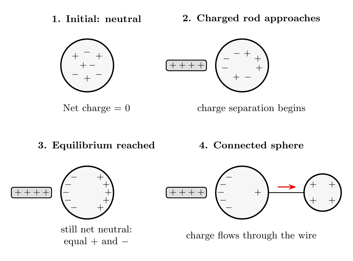
How fast? Basically instantaneous, and the AP exam treats it as taking no time at all, because:
- Each electron only has to shift a tiny distance, so it doesn’t matter that drift speeds in metals are slow.
- The electric field that pushes the electrons spreads through the conductor at nearly the speed of light, so they all start moving at once.
Charging by Induction with a Ground
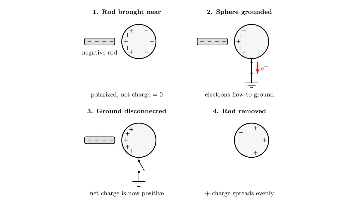
Polarizing a conductor doesn’t give it a net charge. Grounding it while it’s polarized does. Here’s the classic sequence with a negatively charged rod and a neutral metal sphere:
- Bring the rod close (no touching). Electrons in the sphere are pushed to the far side, leaving the near side positive. The sphere is polarized but still neutral.
- Connect the sphere to ground while the rod stays put. Near the negative rod, the sphere sits at a negative potential. Ground holds it at , so electrons flow from the sphere into the ground (the rod repels them, and ground can take as many as needed) until the sphere is back at . The sphere now has a net positive charge.
- Disconnect the ground, still with the rod in place. The electrons that left can’t come back, so the sphere keeps its net positive charge.
- Remove the rod. The positive charge spreads evenly over the sphere’s surface. The sphere ends up with a charge opposite to the rod’s, the rod never touched it, and the rod didn’t lose any of its own charge.
Order matters: if you remove the rod before disconnecting the ground, electrons flow right back up from the ground and the sphere ends up neutral again.
Example: a point charge nC is held 20 cm from the center of a metal sphere of radius 5.0 cm, and the sphere is grounded. How much charge does the ground put on the sphere?
The whole sphere is one equipotential, so its potential equals the potential at its center, and grounding makes that zero. All the induced charge sits on the surface, exactly from the center, so together it contributes at the center no matter how unevenly it’s spread out:
If you then disconnect the ground and take the point charge away, the sphere keeps nC, spread evenly, and its potential becomes V.
Example Problem: Two Connected Spheres
Problem:
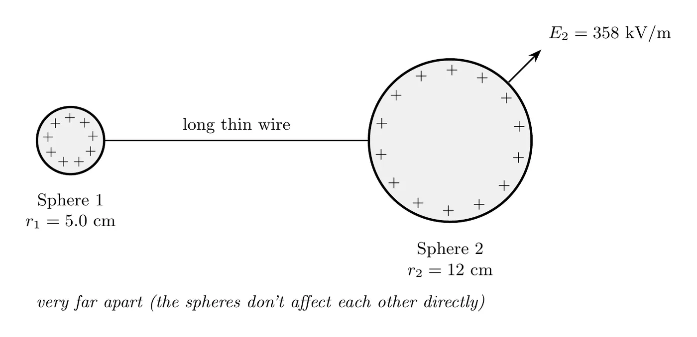
Charge sits on two conducting spheres that are far apart and joined by a long thin wire. The smaller sphere has radius cm and the larger has radius cm. The electric field at the surface of the larger sphere is kV/m.
Find:
(a) The total charge on each sphere.
(b) The surface charge density on each sphere.
Solution
(a) Total Charge on Each Sphere
Step 1: find the charge on the larger sphere (Sphere 2)
Just outside a conducting sphere:
Solve for :
Convert the units first: , and m.
Step 2: find the charge on the smaller sphere (Sphere 1)
They’re connected, so they share a potential:
Answer (a):
- C on the smaller sphere.
- C on the larger sphere.
(b) Surface Charge Density on Each Sphere
Surface charge density is .
For Sphere 1:
For Sphere 2:
Answer (b):
- C/m² on the smaller sphere, which is the higher density.
- C/m² on the larger sphere, the lower density.
Sanity check: , which confirms the smaller sphere packs its charge more densely, exactly as the theory said it would.
Example Problem 2: Sharing a Fixed Amount of Charge
Problem:
Sphere A (radius 2.0 cm) carries nC. Sphere B (radius 4.0 cm) is neutral. The spheres are far apart. You connect them with a long, thin conducting wire. Find the final charge on each sphere and their common potential.
Solution
Two facts fix the answer: charge is conserved, and connected conductors end up at the same potential.
Conservation of charge:
Equal potential (the spheres are far apart, so each acts like an isolated sphere):
Substitute: nC, so nC and nC. The common potential is:
Answer: nC and nC, both at V. (Check: V.)
Which way did charge move? Before the wire, A was at V and B was at 0. Electrons flowed from B to A (toward the higher potential) until the potentials matched. B lost nC worth of electrons, so it ends up at nC, and A drops from nC to nC.
Special case: two identical spheres that touch split the total charge equally, since equal radii at equal potential means equal charge.
Key Physical Insights
Why does the smaller sphere have higher charge density?
Think about the geometry:
- Both spheres sit at the same potential.
- Charge splits up proportionally to radius: .
- But surface area grows faster than that: .
- So .
Charges “crowd” together more on smaller spheres simply because there’s less surface to spread out across.
What Falls Out of It
- Lightning rods. Sharp points have a tiny radius of curvature, so very high charge density and very strong fields, which helps ionize the air.
- Corona discharge. Strong fields near sharp points can break down the air and produce a visible glow.
- Electrical breakdown. Smaller conductors are more likely to discharge at the same voltage.
Proportionality Summary
For two connected conducting spheres:
Double the radius and you:
- Double the charge.
- Halve the charge density.
- Halve the surface field.
Common Mistakes
- Assuming connected conductors carry equal charge. They have equal potential, not equal charge. For spheres, the charge splits up as .
- Thinking the bigger sphere has the higher charge density. It’s the opposite. Smaller radius means higher , since . The small sphere has less total charge but it’s packed in tighter.
- Forgetting to convert units. A field given in kV/m has to become V/m. A radius in cm has to become m. Mixed units are a fast track to a wrong number.
- Confusing charge density with total charge. (charge per area) and (total charge) trend in opposite directions with radius. The bigger sphere has more charge overall but a lower density.
- Underestimating how fast charge redistributes. On conceptual questions, remember it happens nearly instantly (milliseconds or faster) once the conductors are connected. It’s not a slow process.