5.3 - Magnetic Fields of Current-Carrying Wires and the Biot-Savart Law

Introduction to the Biot-Savart Law

The Biot-Savart Law lets you calculate or derive expressions for magnetic fields created by electric currents flowing through wires. It’s analogous to Coulomb’s Law for electric fields, but it applies to moving charges (currents).

Its purpose: to determine the magnitude and direction of the magnetic field a current-carrying wire creates at any point in space.

The Biot-Savart Law Equation

General Form

d\vec{B} = \frac{\mu_0}{4\pi} \frac{I d\vec{\ell} \times \hat{r}}{r^2}

where: -

d\vec{B}

= infinitesimal magnetic field contribution (T) -

\mu_0 = 4\pi \times 10^{-7}

T·m/A, the permeability of free space -

I

= current through the wire (A) -

d\vec{\ell}

= infinitesimal length element of wire (a vector pointing in the current direction) -

\hat{r}

= unit vector pointing from the wire element to the observation point -

r

= distance from the wire element to the observation point (m) -

\times

= cross product

Understanding the Components

$\mu_0$ (mu-naught): the magnetic permeability constant that shows up in every magnetic field equation.

$I$ : the current flowing through the wire, constant for a given wire.

$d\ell$ : a small segment of wire, and this is what you integrate over.

$\hat{r}$ (r-hat): a unit vector with magnitude 1, pointing radially from the wire element toward the observation point.

$r$ : the distance from the wire element to the observation point.

Magnitude Form

For practical calculations, the magnitude is:

dB = \frac{\mu_0}{4\pi} \frac{I \, d\ell \sin\theta}{r^2}

where

\theta

is the angle between

d\vec{\ell}

and

\hat{r}

An important simplification: when

d\vec{\ell}

is perpendicular to

\hat{r}

, which happens a lot,

\sin\theta = 1

, so:

dB = \frac{\mu_0 I \, d\ell}{4\pi r^2}

To find the total magnetic field, integrate over the whole wire:

\vec{B} = \int d\vec{B} = \frac{\mu_0 I}{4\pi} \int \frac{d\vec{\ell} \times \hat{r}}{r^2}

Magnetic Field Pattern Around a Wire

The magnetic field vectors around a current-carrying wire are tangent to concentric circles centered on the wire.

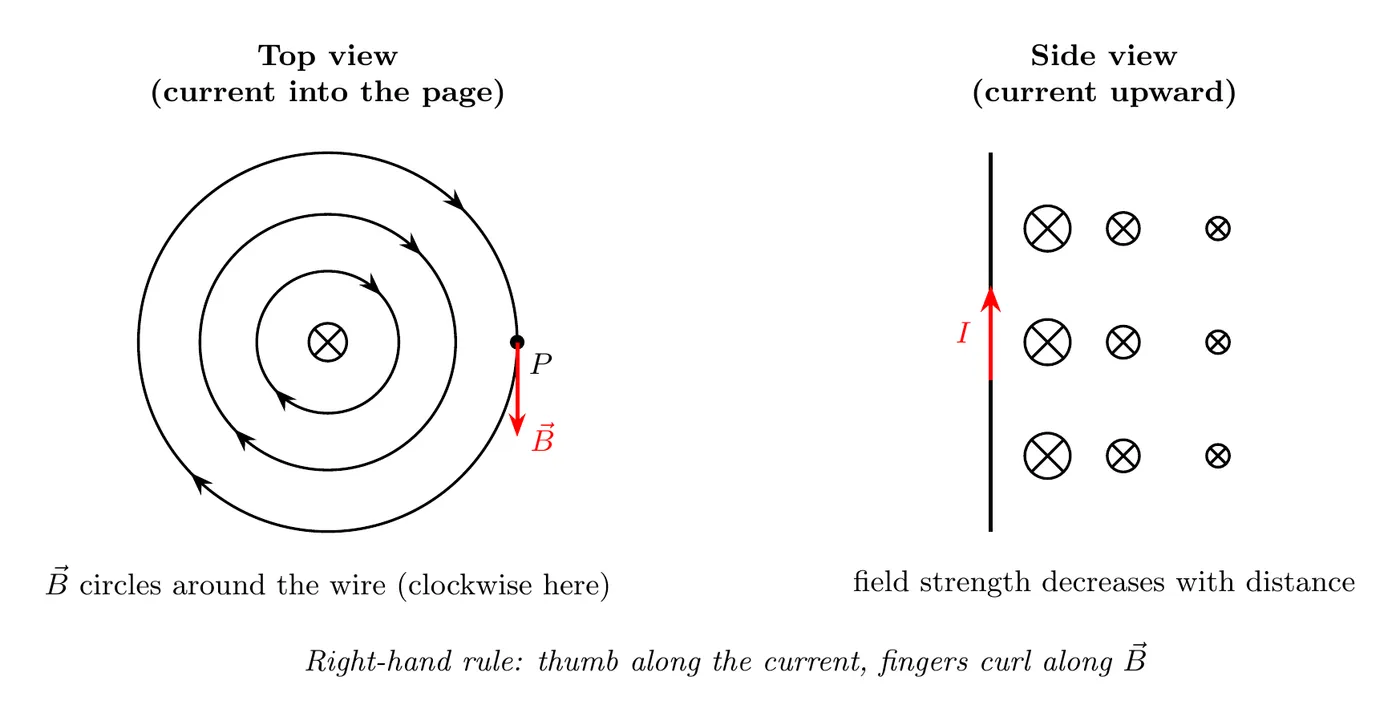
5.3 - Magnetic Fields of Current-Carrying Wires and the Biot-Savart Law

The right-hand rule for a wire: - Point your thumb in the direction of the current. - Your fingers curl in the direction of the magnetic field circles.

The field has no component toward or away from the wire and no component parallel to the wire. It only wraps around. That comes straight from the cross product in the Biot-Savart Law:

d\vec{B}

is perpendicular to both

d\vec{\ell}

(which runs along the wire) and

\hat{r}

(which points from the wire out to the point), and the only direction perpendicular to both is around the wire.

Magnetic Field from a Current Loop

A special and important case is a circular loop of wire carrying current.

Formula for the Center of a Loop

At the center of a circular loop of radius

R

carrying current

I

B = \frac{\mu_0 I}{2R}

This comes from integrating the Biot-Savart Law around the entire loop (angle

\theta = 2\pi

), as you’ll see in the example problem.

Only the Biot-Savart Law itself is on the AP equation sheet, not this result, so be ready to derive it.

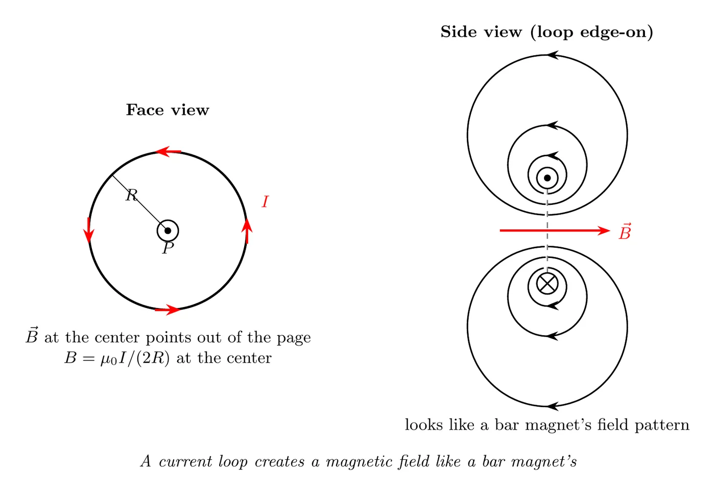
A physical insight: a current loop acts like a magnetic dipole, with a field pattern very similar to a bar magnet’s.

Force on a Current-Carrying Wire

A current-carrying wire sitting in an external magnetic field feels a force.

Formula

\vec{F}_B = I\vec{\ell} \times \vec{B}

For a wire segment of length

\ell

F_B = I\ell B\sin\theta

where

\theta

is the angle between the wire (the current direction) and the magnetic field.

For a curved wire or a varying field, integrate over the wire:

\vec{F}_B = \int I \, d\vec{\ell} \times \vec{B}

Maximum force: when the wire is perpendicular to the field (

\theta = 90°

F = I\ell B

No force: when the wire is parallel to the field (

\theta = 0°

F = 0

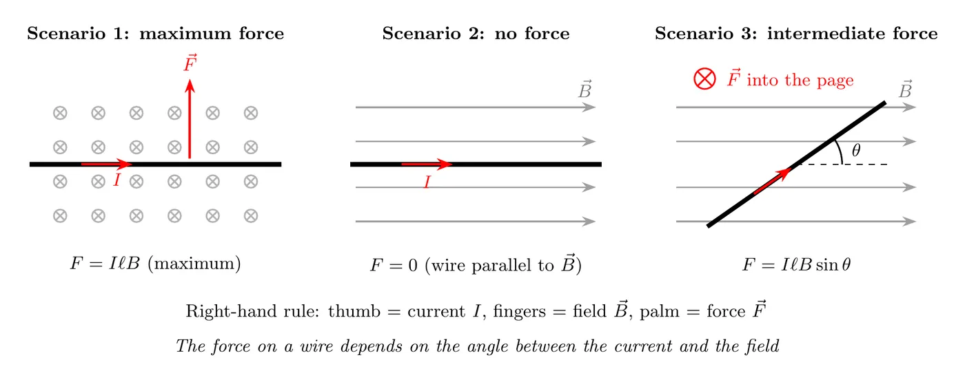
Uniform field shortcut. In a uniform field, a curved wire feels the same net force as a straight wire running between its two ends with the same current. For example, a semicircle of radius

R

lying in the page, with

\vec{B}

perpendicular to the page, feels

F = I(2R)B

, the same as its straight diameter. You need the integral

\vec{F}_B = \int I\,d\vec{\ell} \times \vec{B}

when the field changes along the wire:

Example: Force in a Field That Isn’t Uniform

Problem: A long straight wire carries

I_1 = 20

A up the page. A 0.080 m rod lies in the page perpendicular to the long wire, with its near end 0.020 m from the wire and its far end 0.10 m away. The rod carries

I_2 = 5.0

A away from the long wire. Find the magnetic force on the rod.

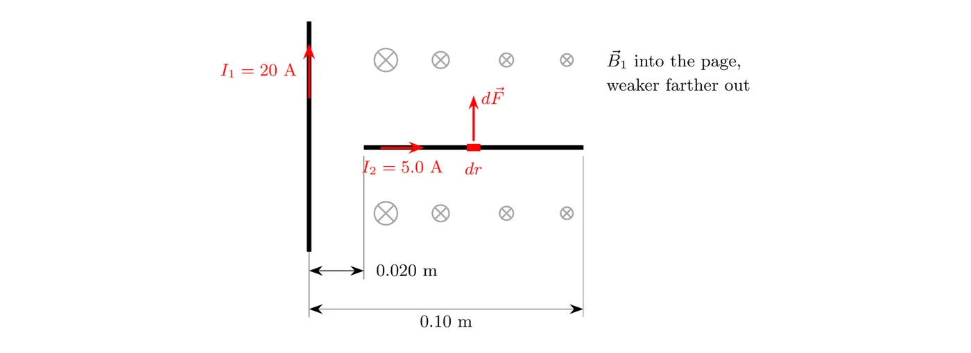
The long wire’s field,

B_1 = \frac{\mu_0 I_1}{2\pi r}

(into the page on the rod’s side), gets weaker along the rod, so you can’t just use

F = I\ell B

. Cut the rod into pieces

dr

. Each piece is perpendicular to

\vec{B}_1

, so

dF = I_2B_1\,dr

F = \int_{0.020}^{0.10} I_2\frac{\mu_0 I_1}{2\pi r}\,dr = \frac{\mu_0 I_1 I_2}{2\pi}\ln\frac{0.10}{0.020}

F = (2.0 \times 10^{-7}\text{ T·m/A})(20 \text{ A})(5.0 \text{ A})\ln 5.0 = 3.2 \times 10^{-5} \text{ N}

Direction:

d\vec{\ell}

points away from the wire (

\hat{i}

) and

\vec{B}_1

points into the page (

-\hat{k}

), and

\hat{i} \times (-\hat{k}) = +\hat{j}

. The force points up the page, parallel to the long wire’s current.

Force Between Two Parallel Wires

Each wire sits in the magnetic field of the other, so two current-carrying wires push or pull on each other. Wire 1’s field at wire 2, a distance

d

away, is

B_1 = \frac{\mu_0 I_1}{2\pi d}

, and it’s perpendicular to wire 2. So the force on a length

\ell

of wire 2 is

F = I_2\ell B_1 = \frac{\mu_0 I_1 I_2 \ell}{2\pi d}

Wire 2 pulls on wire 1 with the same size force in the opposite direction (Newton’s third law). - Currents in the same direction attract. - Currents in opposite directions repel.

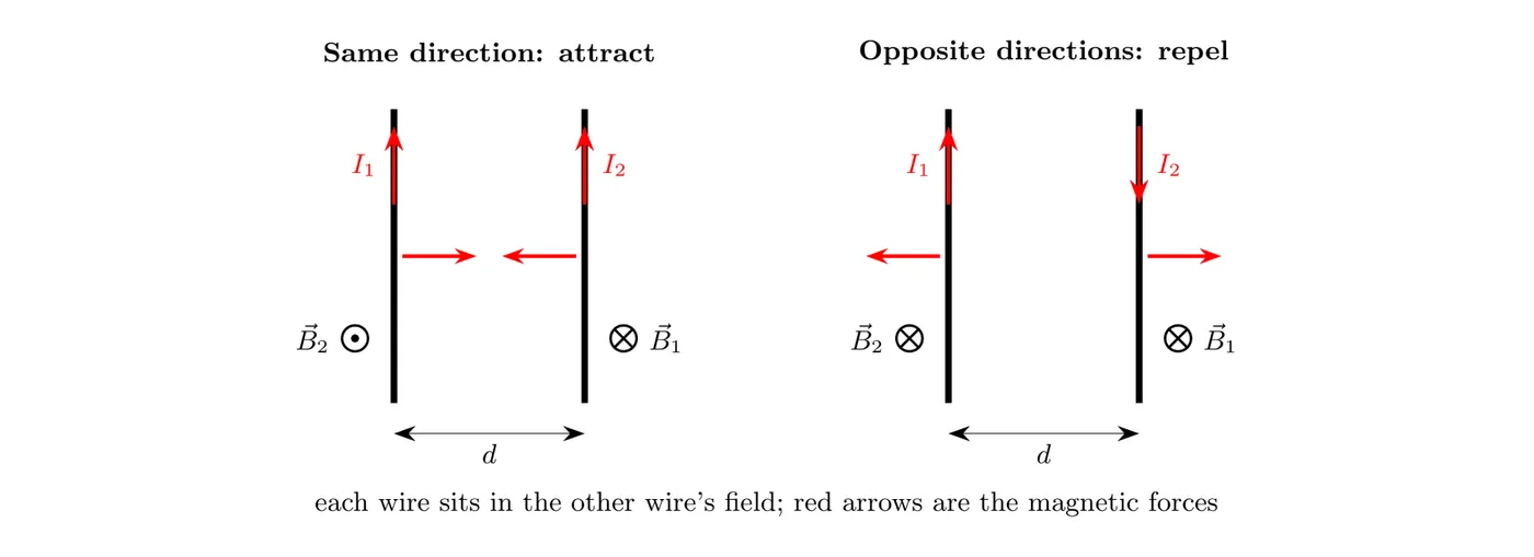
Example. Two long parallel wires 4.0 cm apart carry 8.0 A and 5.0 A in the same direction. Find the force on a 0.50 m length of either wire.

F = \frac{(4\pi \times 10^{-7}\text{ T·m/A})(8.0 \text{ A})(5.0 \text{ A})(0.50 \text{ m})}{2\pi(0.040 \text{ m})} = 1.0 \times 10^{-4} \text{ N}

Example Problem: Magnetic Field at the Center of a Circular Arc

Problem: A wire carrying current

I

forms a circular arc with radius

R

, sweeping through an arbitrary angle

\theta

(in radians). Derive an expression for the magnetic field at the center of the arc (point P).

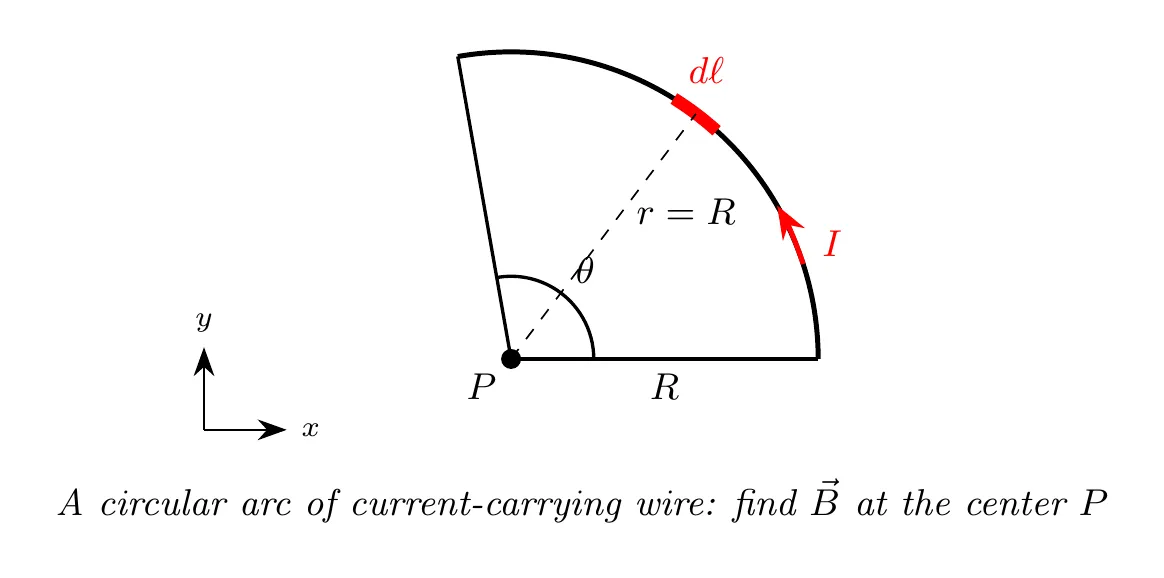
Solution

Step 1: Start with the Biot-Savart Law

d\vec{B} = \frac{\mu_0}{4\pi} \frac{I \, d\vec{\ell} \times \hat{r}}{r^2}

Step 2: Identify the constants

For this geometry: - The current

I

is constant. - The distance from any point on the arc to the center is

r = R

, also constant. - The wire element

d\vec{\ell}

is always perpendicular to

\hat{r}

(the radial direction). - So

|d\vec{\ell} \times \hat{r}| = d\ell

, since

\sin 90° = 1

Step 3: Set up the integral

Since

\mu_0/(4\pi)

I

, and

R

are all constants, factor them out:

B = \frac{\mu_0 I}{4\pi R^2} \int d\ell

Step 4: Express $d\ell$ in terms of the angle

For a circular arc,

d\ell = R \, d\theta

The arc runs from

0

\theta

, the total angle swept:

B = \frac{\mu_0 I}{4\pi R^2} \int_0^\theta R \, d\theta

Step 5: Simplify

B = \frac{\mu_0 I}{4\pi R^2} \cdot R \int_0^\theta d\theta

B = \frac{\mu_0 I}{4\pi R} \int_0^\theta d\theta

Step 6: Integrate

\int_0^\theta d\theta = [\theta]_0^\theta = \theta - 0 = \theta

Step 7: Final answer

\boxed{B = \frac{\mu_0 I \theta}{4\pi R}}

The physical read: the magnetic field at the center is proportional to - the current

I

, so more current means a stronger field, - the angle

\theta

, so a bigger arc means a stronger field, and inversely proportional to the radius

R

, so a bigger radius means a weaker field at the center.

Special Case: The Complete Loop

For a complete circular loop, the angle swept is

\theta = 2\pi

radians (360°).

Substitute

\theta = 2\pi

into the result:

B = \frac{\mu_0 I (2\pi)}{4\pi R}

B = \frac{2\mu_0 I}{4R}

B = \frac{\mu_0 I}{2R}

That confirms the complete-loop formula from earlier.

This shows the power of the general result: the formula

B = \frac{\mu_0 I\theta}{4\pi R}

works for any arc angle, and the complete loop is just the special case where

\theta = 2\pi

Example Problem: Field on the Perpendicular Bisector of a Straight Wire

Problem: A straight wire of length

L

carries current

I

. Derive the magnetic field at point P, a distance

a

from the wire’s midpoint along the perpendicular bisector.

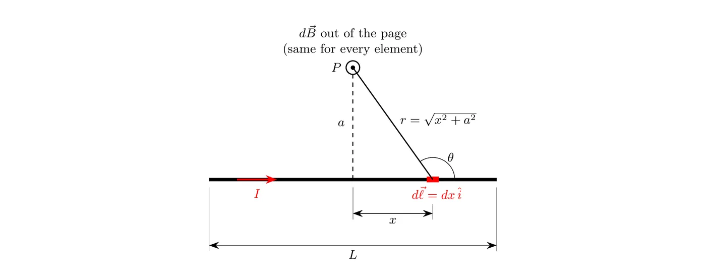
Solution

Step 1: Set up one piece

Put the wire on the

x

-axis from

-L/2

L/2

, with P a height

a

above the middle. A piece

dx

at position

x

is a distance

r = \sqrt{x^2 + a^2}

from P, and the angle

\theta

between

d\vec{\ell}

and

\hat{r}

has

\sin\theta = \frac{a}{r}

. So the Biot-Savart Law gives

dB = \frac{\mu_0}{4\pi}\frac{I\,dx\sin\theta}{r^2} = \frac{\mu_0 I}{4\pi}\frac{a\,dx}{(x^2 + a^2)^{3/2}}

Step 2: Check the direction

With the current to the right and P above the wire,

d\vec{\ell} \times \hat{r}

points out of the page for every piece. Since every

d\vec{B}

points the same way, you can add the magnitudes directly.

Step 3: Integrate

B = \frac{\mu_0 I a}{4\pi}\int_{-L/2}^{L/2}\frac{dx}{(x^2 + a^2)^{3/2}} = \frac{\mu_0 I a}{4\pi}\left[\frac{x}{a^2\sqrt{x^2 + a^2}}\right]_{-L/2}^{L/2}

(That integral comes from the substitution

x = a\tan\phi

, or a table of integrals.) Plugging in the limits and simplifying:

\boxed{B = \frac{\mu_0 I L}{2\pi a\sqrt{L^2 + 4a^2}}}

Step 4: Check the limit

For a very long wire (

L \gg a

\sqrt{L^2 + 4a^2} \approx L

, and the result becomes

B = \frac{\mu_0 I}{2\pi a}

, the infinite-wire field from Topic 5.4. Even a fairly short wire gets close: with

L = 4a

, the field is

\frac{4}{\sqrt{20}} = 0.89

of the infinite-wire value, because the far ends of a wire contribute very little at P.

Example Problem: Field on the Axis of a Circular Loop

Problem: A circular loop of radius

R

carries current

I

. Derive the magnetic field at point P on the loop’s central axis, a distance

x

from its center.

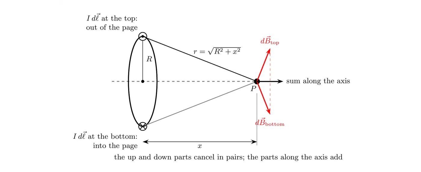
Solution

Step 1: One piece of the loop

Every piece

d\ell

of the loop is the same distance from P,

r = \sqrt{R^2 + x^2}

, and

d\vec{\ell}

is always perpendicular to

\hat{r}

(so

\sin\theta = 1

dB = \frac{\mu_0}{4\pi}\frac{I\,d\ell}{R^2 + x^2}

Step 2: Use symmetry

Each

d\vec{B}

is perpendicular to its own

\vec{r}

, so it tilts away from the axis. The piece on the opposite side of the loop makes a

d\vec{B}

tilted the other way, so the parts perpendicular to the axis cancel in pairs. Only the parts along the axis survive. Since

d\vec{B}

is perpendicular to

\vec{r}

, similar triangles give the part along the axis as

dB

times

\frac{R}{\sqrt{R^2 + x^2}}

dB_x = \frac{\mu_0 I\,d\ell}{4\pi(R^2 + x^2)} \cdot \frac{R}{\sqrt{R^2 + x^2}} = \frac{\mu_0 I R\,d\ell}{4\pi(R^2 + x^2)^{3/2}}

Step 3: Integrate around the loop

Everything except

d\ell

is constant, and

\oint d\ell = 2\pi R

B = \frac{\mu_0 I R}{4\pi(R^2 + x^2)^{3/2}}(2\pi R) \quad\Rightarrow\quad \boxed{B = \frac{\mu_0 I R^2}{2(R^2 + x^2)^{3/2}}}

The field points along the axis, the way your thumb points when your fingers curl with the current.

Step 4: Check the limits - At the center (

x = 0

B = \frac{\mu_0 I R^2}{2R^3} = \frac{\mu_0 I}{2R}

, which matches the loop formula above. - One radius out (

x = R

B = \frac{\mu_0 I R^2}{2(2R^2)^{3/2}} = \frac{B_{center}}{2^{3/2}}

, about 35% of the value at the center. - Far away (

x \gg R

B \approx \frac{\mu_0 I R^2}{2x^3}

. The field drops off as

1/x^3

, just like a magnetic dipole’s field (Topic 5.1).

Example Problem: Combining Arcs and Straight Segments

Problem: A loop is made of two quarter circles that share the same center P, with radii

R_1 = 0.10

m and

R_2 = 0.20

m, joined by two straight radial pieces. It carries 4.0 A, counterclockwise around the outer arc and clockwise around the inner arc. Find the magnetic field at P.

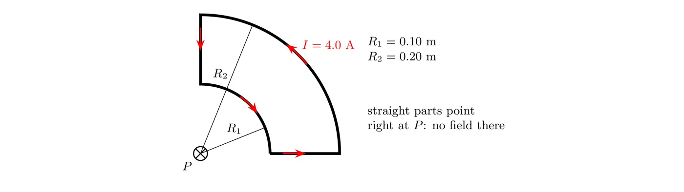
Use superposition: find the field from each piece at P, then add them as vectors. - Straight pieces: they point straight at P, so

d\vec{\ell}

is parallel to

\hat{r}

and

d\vec{\ell} \times \hat{r} = 0

. They add nothing at P. - Outer arc: a quarter circle has

\theta = \frac{\pi}{2}

, so

B_2 = \frac{\mu_0 I(\pi/2)}{4\pi R_2} = \frac{\mu_0 I}{8R_2}

, out of the page (counterclockwise current). - Inner arc:

B_1 = \frac{\mu_0 I}{8R_1}

, into the page (clockwise current).

B = \frac{\mu_0 I}{8}\left(\frac{1}{R_1} - \frac{1}{R_2}\right) = \frac{(4\pi \times 10^{-7}\text{ T·m/A})(4.0 \text{ A})}{8}\left(\frac{1}{0.10 \text{ m}} - \frac{1}{0.20 \text{ m}}\right) = 3.1 \times 10^{-6} \text{ T}

The net field points into the page, because the inner arc is closer to P and wins.

Common Current Configurations

Using the Biot-Savart Law, you can derive the magnetic fields for various wire setups:

Configuration	Magnetic Field	Location
Straight infinite wire	$B = \frac{\mu_0 I}{2\pi r}$	Distance $r$ from wire
Straight wire of length $L$	$B = \frac{\mu_0 I L}{2\pi a\sqrt{L^2 + 4a^2}}$	Distance $a$ from the midpoint, on the perpendicular bisector
Circular loop	$B = \frac{\mu_0 I}{2R}$	Center of loop (radius $R$ )
Circular loop (on its axis)	$B = \frac{\mu_0 I R^2}{2(R^2 + x^2)^{3/2}}$	Distance $x$ from the center, along the axis
Circular arc (angle $\theta$ )	$B = \frac{\mu_0 I\theta}{4\pi R}$	Center of arc
Solenoid (coil)	$B = \mu_0 n I$	Inside a long solenoid ( $n$ = turns per length)

Note: the straight infinite wire formula gets derived using Ampère’s Law in the next topic.

Right-Hand Rules Summary

For Magnetic Field from Current (Biot-Savart)

Straight wire: - Thumb: points in the current direction. - Fingers: curl in the direction of the magnetic field circles.

Current loop: - Fingers: curl in the direction of the current around the loop. - Thumb: points in the direction of the magnetic field through the center.

For Force on Current in a Field

Wire in an external field: - Thumb: current direction (

I

). - Fingers: field direction (

\vec{B}

). - Palm: force direction (

\vec{F}

Preview: Ampère’s Law

In the next topic, we’ll get into Ampère’s Law, which gives you an alternative and often simpler way to calculate magnetic fields when there’s enough symmetry.

Ampère’s Law:

\oint \vec{B} \cdot d\vec{\ell} = \mu_0 I_{enclosed}

With Maxwell’s addition (a term for changing electric fields, covered in the next topic), this becomes the fourth of Maxwell’s equations. Ampère’s Law is especially useful for: - Long straight wires. - Solenoids. - Toroids. - Any configuration with cylindrical or planar symmetry.

Ampère’s Law relates to Biot-Savart the same way Gauss’s Law relates to Coulomb’s Law. Both give you the same answers, but Ampère’s Law is far easier when symmetry is present.

Summary of Key Formulas

Biot-Savart Law

d\vec{B} = \frac{\mu_0}{4\pi} \frac{I \, d\vec{\ell} \times \hat{r}}{r^2}

Magnetic Field Magnitudes

B_{arc} = \frac{\mu_0 I\theta}{4\pi R} \quad \text{(arc at center)}

B_{loop} = \frac{\mu_0 I}{2R} \quad \text{(complete loop at center)}

Force on a Wire

\vec{F}_B = I\vec{\ell} \times \vec{B}

F_B = I\ell B\sin\theta

Common Mistakes

Forgetting the cross product in Biot-Savart. The $d\vec{\ell} \times \hat{r}$ term means the field depends on the angle between the wire element and the radius vector. When they’re perpendicular (the common case), it simplifies, but don’t forget it’s there.

Using the wrong angle in the arc formula. The angle $\theta$ in $B = \frac{\mu_0 I\theta}{4\pi R}$ has to be in radians, not degrees. A semicircle is $\theta = \pi$ , not $\theta = 180$ .

Confusing radius R with distance r. In the arc problem, $r = R$ , since the distance from the wire to the center equals the arc radius. But in general problems with arbitrary observation points, $r$ varies and isn’t the same as the geometric radius.

Using the wrong right-hand rule. To find B from a current, curl your fingers in the current direction with your thumb showing the field direction (for loops), or point your thumb in the current direction with your fingers curling for the field circles (for straight wires). Don’t confuse this with the force rule.

Forgetting that the constants are constant during integration. When you integrate Biot-Savart, $\mu_0$ , $4\pi$ , $I$ , and often $R$ (for circular geometry) are constants you can factor out. Pull them out early to simplify the integral.

Back Next