5.4 - Ampère’s Law

Introduction to Ampère’s Law

Ampère’s Law relates the magnitude of a magnetic field to the current enclosed by an imaginary closed path called an Amperian loop. It’s the magnetic analog of Gauss’s Law for electric fields.

The comparison: - Gauss’s Law uses a closed surface (a Gaussian surface) to relate the electric field to the enclosed charge. - Ampère’s Law uses a closed path (an Amperian loop) to relate the magnetic field to the enclosed current.

When to use Ampère’s Law: - High-symmetry situations (cylindrical, planar, solenoid). - Calculating magnetic fields around current-carrying wires. - It’s much simpler than Biot-Savart when symmetry exists.

Ampère’s Law Formula

Basic Statement

\oint \vec{B} \cdot d\vec{\ell} = \mu_0 I_{enclosed}

where: -

\oint

= line integral around a closed path (the Amperian loop) -

\vec{B}

= magnetic field vector (T) -

d\vec{\ell}

= infinitesimal path element along the loop -

\mu_0 = 4\pi \times 10^{-7}

T·m/A, the permeability of free space -

I_{enclosed}

= total current passing through the area enclosed by the loop (A)

The physical meaning: the circulation of the magnetic field around a closed loop equals

\mu_0

times the current threading through that loop.

Comparison to Gauss’s Law

Gauss’s Law (Electric)	Ampère’s Law (Magnetic)
$\oint \vec{E} \cdot d\vec{A} = \frac{Q_{enclosed}}{\epsilon_0}$	$\oint \vec{B} \cdot d\vec{\ell} = \mu_0 I_{enclosed}$
Surface integral	Line integral
Encloses charge	Encloses current
Relates to $\epsilon_0$	Relates to $\mu_0$

Applications of Ampère’s Law

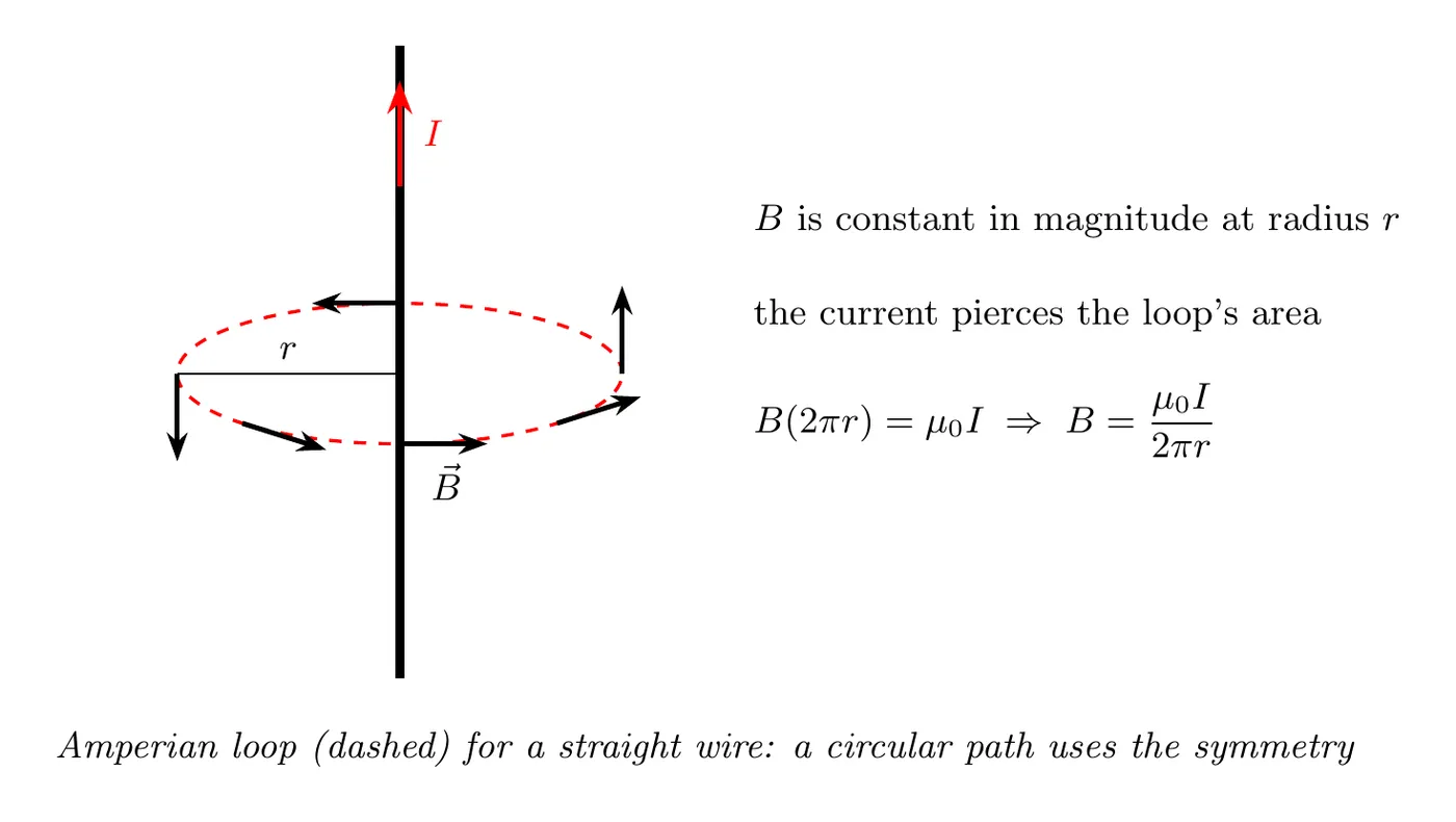
Long Straight Wire

For an infinitely long straight wire carrying current

I

B = \frac{\mu_0 I}{2\pi r}

where

r

is the perpendicular distance from the wire.

Deriving it with Ampère’s Law: - Choose a circular Amperian loop of radius

r

centered on the wire. - By symmetry,

B

is constant along the loop and tangent to it. -

\oint \vec{B} \cdot d\vec{\ell} = B(2\pi r)

. -

I_{enclosed} = I

. - So

B(2\pi r) = \mu_0 I

. - Result:

B = \frac{\mu_0 I}{2\pi r}

B_{\text{wire}} = \frac{\mu_0 I}{2\pi r}

isn’t on the AP equation sheet (Ampère’s Law is), so be ready to derive it with the steps above.

Example. A long straight wire carries 15 A. Find the magnetic field 3.0 cm from it.

B = \frac{\mu_0 I}{2\pi r} = \frac{(4\pi \times 10^{-7}\text{ T·m/A})(15 \text{ A})}{2\pi(0.030 \text{ m})} = 1.0 \times 10^{-4} \text{ T}

That’s about twice Earth’s field (about 50 μT), which is why a compass needle near a current-carrying wire swings noticeably toward the circles around the wire. Double the distance to 6.0 cm and the field halves to

5.0 \times 10^{-5}

T, since

B \propto \frac{1}{r}

Solenoid (Long Coil)

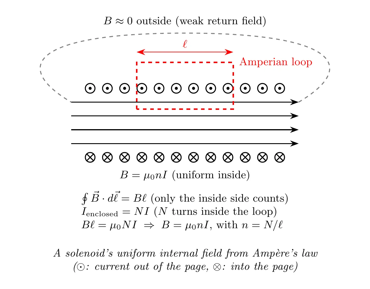
A solenoid is a long coil of wire. Inside a very long solenoid, the magnetic field is uniform and parallel to the axis.

The magnetic field inside an ideal solenoid:

B = \mu_0 n I

where: -

n

= turn density, the number of turns per unit length (turns/m) -

I

= current through the wire (A)

An alternative form:

B = \frac{\mu_0 N I}{L}

where: -

N

= total number of turns -

L

= length of the solenoid -

n = N/L

Key properties: - Inside: a strong, uniform field parallel to the axis. - Outside: a negligible field, ideally zero for an infinite solenoid.

Deriving the Solenoid Field

Unless a problem says otherwise, treat every solenoid as very long: the field inside is uniform and along the axis, and the field outside is negligible. Then use a rectangular Amperian loop with one long side (length

\ell

) inside the solenoid, parallel to the axis, and the other long side outside: - Inside side:

\vec{B}

is parallel to the path, so it contributes

B\ell

. - Outside side:

B \approx 0

, so it contributes nothing. - The two short sides: inside the solenoid

\vec{B}

is perpendicular to them, and outside

B \approx 0

, so they contribute nothing.

N

turns pass through the loop, each carrying

I

, the enclosed current is

NI

B\ell = \mu_0 NI \quad\Rightarrow\quad B = \mu_0\frac{N}{\ell}I = \mu_0 nI

The answer doesn’t depend on where you put the inside side of the loop, which is why the field is the same everywhere inside.

Example. A solenoid 0.30 m long has 600 turns and carries 2.5 A. Find the field inside.

B = \mu_0 nI = (4\pi \times 10^{-7}\text{ T·m/A})\left(\frac{600}{0.30 \text{ m}}\right)(2.5 \text{ A}) = 6.3 \times 10^{-3} \text{ T}

Squeeze the same 600 turns into 0.15 m and

n

doubles, so

B

doubles too. The solenoid’s radius doesn’t show up anywhere.

Maxwell’s Addition: The Ampère-Maxwell Law

The complete form of Ampère’s Law includes a term James Clerk Maxwell added, which makes it the Ampère-Maxwell Law, the fourth of Maxwell’s equations.

Complete Form

\oint \vec{B} \cdot d\vec{\ell} = \mu_0 I_{enclosed} + \mu_0\epsilon_0\frac{d\Phi_E}{dt}

The extra term

\mu_0\epsilon_0\frac{d\Phi_E}{dt}

accounts for displacement current from changing electric fields.

Maxwell’s contribution is that second term:

\mu_0\epsilon_0\frac{d\Phi_E}{dt}

The physical meaning: a changing electric flux, even with no actual current, can create a magnetic field. That term is essential for: - Electromagnetic waves. - Understanding light as electromagnetic radiation. - Completing the symmetry between electricity and magnetism.

Historically, Maxwell’s addition of this term predicted electromagnetic waves and unified electricity, magnetism, and light into a single theory.

Where you’d see it: a capacitor that’s charging. Current flows in the wires, but no charge crosses the gap between the plates. The electric field in the gap is growing, though, and that changing electric field makes a magnetic field that circles the gap, just like the field circling the wires.

On the AP exam, you won’t calculate with the

\mu_0\epsilon_0\frac{d\Phi_E}{dt}

term, but you do need to know that a changing electric field creates a magnetic field, similar to the way a current does.

Example Problem: Magnetic Field Inside and Outside an Infinite Cylinder

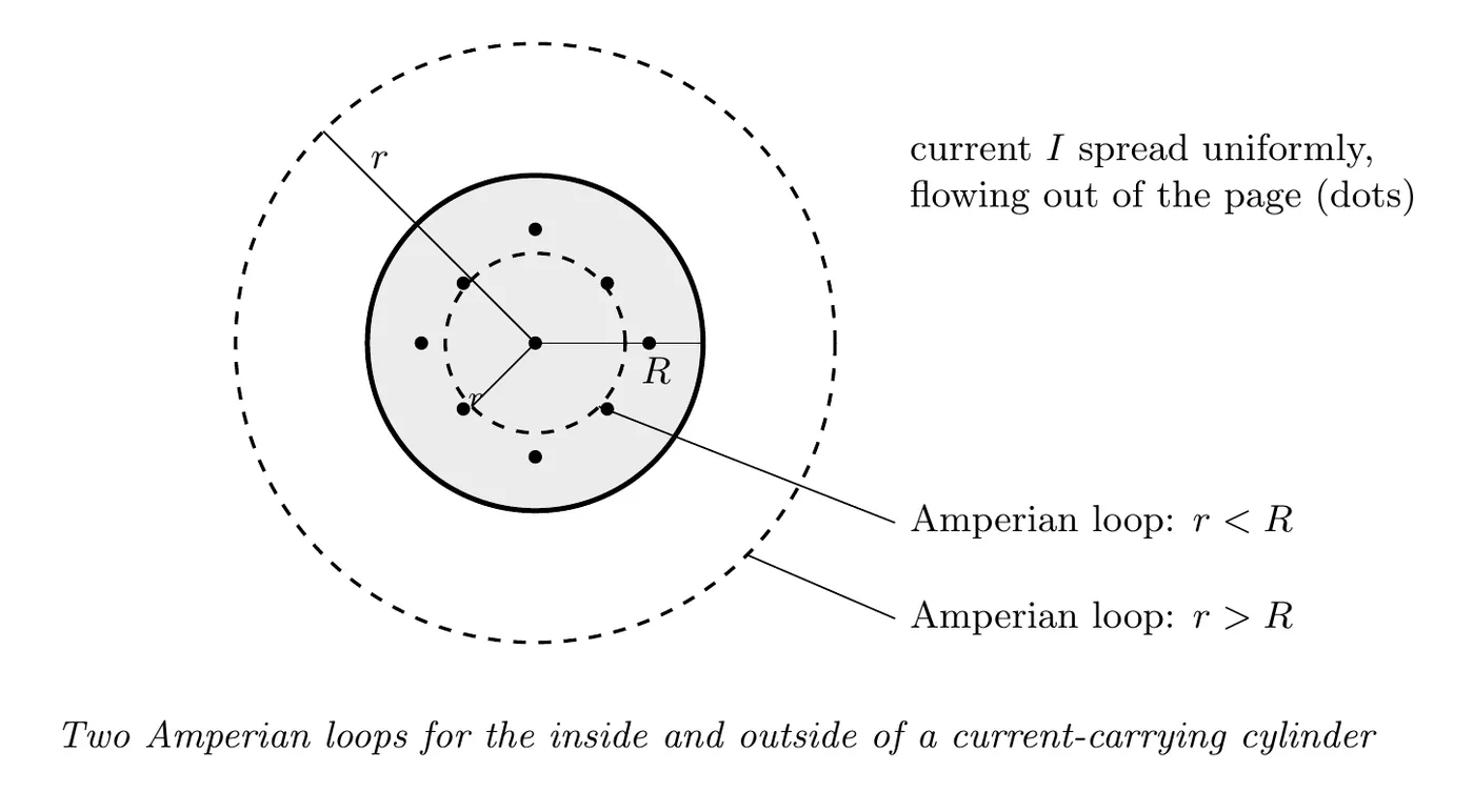
Problem: A long solid cylindrical conductor of radius

R

carries a uniformly distributed current

I

. Use Ampère’s Law to derive expressions for the magnetic field:

Outside the cylinder (at distance $r > R$ from the axis).

Inside the cylinder (at distance $r < R$ from the axis).

Solution

Part (a): Outside the cylinder (r > R)

Step 1: Choose the Amperian loop

Pick a circular path of radius

r > R

centered on the cylinder axis.

Step 2: Apply Ampère’s Law

\oint \vec{B} \cdot d\vec{\ell} = \mu_0 I_{enclosed}

Step 3: Evaluate the left side

By cylindrical symmetry,

B

is constant along the loop and tangent to it:

\oint \vec{B} \cdot d\vec{\ell} = B \oint d\ell = B(2\pi r)

Step 4: Find the enclosed current

The entire cylinder is enclosed, so:

I_{enclosed} = I

Step 5: Solve for B

B(2\pi r) = \mu_0 I

\boxed{B = \frac{\mu_0 I}{2\pi r}}

The physical read: outside the cylinder, the field is the same as for an infinitely thin wire carrying the same current. It falls off as

1/r

Part (b): Inside the cylinder (r < R)

Step 1: Choose the Amperian loop

Pick a circular path of radius

r < R

centered on the cylinder axis.

Step 2: Find the enclosed current

Only a fraction of the total current is enclosed. Since the current is uniformly distributed, use the current density:

J = \frac{I}{A_{cylinder}} = \frac{I}{\pi R^2}

The current enclosed by a loop of radius

r

I_{enclosed} = J \cdot A_{loop} = \frac{I}{\pi R^2} \cdot \pi r^2

I_{enclosed} = I\frac{r^2}{R^2}

Step 3: Apply Ampère’s Law

\oint \vec{B} \cdot d\vec{\ell} = \mu_0 I_{enclosed}

B(2\pi r) = \mu_0 I\frac{r^2}{R^2}

Step 4: Solve for B

B = \frac{\mu_0 I r^2}{2\pi r R^2}

\boxed{B = \frac{\mu_0 I r}{2\pi R^2}}

The physical read: inside the cylinder, the field grows linearly with distance from the axis (

B \propto r

). At the center (

r = 0

), the field is zero.

Magnetic Field Profile: Inside vs. Outside

The complete magnetic field profile behaves very differently in the two regions.

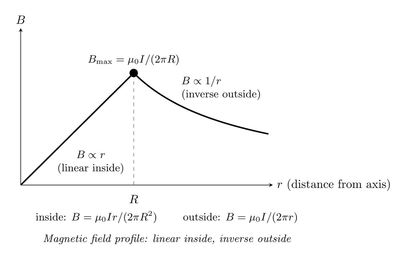
Key observations: - At the center (

r = 0

B = 0

. - Inside (

0 < r < R

B

increases linearly with

r

. - At the surface (

r = R

B

is at its maximum,

\frac{\mu_0 I}{2\pi R}

. - Outside (

r > R

B

decreases as

\frac{1}{r}

. - The field is continuous at the surface, with no jump.

Compared to the electric field in a uniformly charged sphere: - The mathematical structure is the same: linear inside, inverse-power outside. - It reveals a deep parallel between E and B field distributions.

Example Problem: A Thick Slab of Current

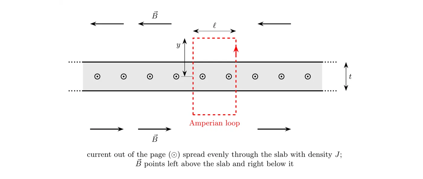
Problem: A very wide, flat conducting slab of thickness

t

carries current out of the page, spread evenly with current density

J

. Use Ampère’s Law to find the magnetic field outside the slab, and inside it at a distance

y

from the middle plane.

Solution

Step 1: Use the symmetry

Think of the slab as lots of wires side by side, all with current out of the page. Above the slab their fields add up to point left, and below it they point right. The field is parallel to the slab, and its size depends only on the distance from the middle plane, the same above and below.

Step 2: Choose the Amperian loop

Use a rectangle that straddles the slab, with its top and bottom sides (length

\ell

) parallel to the slab at a distance

y

above and below the middle. Go around it counterclockwise: - Top and bottom sides: on the top you travel left, the same way

\vec{B}

points, and on the bottom you travel right, again with

\vec{B}

. Each contributes

B\ell

. - The two sides that cross the slab:

\vec{B}

is perpendicular to them, so they contribute nothing.

\oint \vec{B} \cdot d\vec{\ell} = 2B\ell

Step 3: Outside the slab (

y > t/2

)

The loop encloses the full thickness, so

I_{enclosed} = J(t\ell)

2B\ell = \mu_0 Jt\ell \quad\Rightarrow\quad \boxed{B = \frac{\mu_0 Jt}{2}}

The field outside doesn’t depend on distance: as long as the slab is much wider than your distance from it, the field is the same close to the slab or farther out.

Step 4: Inside the slab (

y < t/2

)

Now the loop encloses only a thickness

2y

, so

I_{enclosed} = J(2y\ell)

2B\ell = \mu_0 J(2y)\ell \quad\Rightarrow\quad \boxed{B = \mu_0 Jy}

The field grows linearly from zero at the middle plane to

\frac{\mu_0 Jt}{2}

at the surfaces, where it matches the outside value.

Example Problem: A Cylinder with Non-Uniform Current Density

Problem: A long solid wire of radius

R = 2.0

mm carries a total current

I = 12

A along its length, but the current isn’t spread evenly. The current density grows with distance from the axis as

J = br

, where

b

is a constant. Find

B

inside the wire at

r = 1.0

mm.

Step 1: Enclosed current. When

J

changes with

r

, add it up over thin rings of area

dA = 2\pi r'\,dr'

(Topic 4.1):

I_{enclosed} = \int_0^r J\,dA = \int_0^r br'(2\pi r'\,dr') = \frac{2\pi br^3}{3}

Step 2: Use the total current. At

r = R

, the loop encloses all of it, so

I = \frac{2\pi bR^3}{3}

. Dividing the two results gives a handy shortcut:

\frac{I_{enclosed}}{I} = \frac{r^3}{R^3}

Step 3: Ampère’s Law with a circular loop of radius

r

B(2\pi r) = \mu_0 I\frac{r^3}{R^3} \quad\Rightarrow\quad B = \frac{\mu_0 I r^2}{2\pi R^3}

Step 4: Plug in the numbers. At

r = 1.0

mm,

I_{enclosed} = (12 \text{ A})\left(\frac{1.0}{2.0}\right)^3 = 1.5

A, so

B = \frac{\mu_0 I_{enclosed}}{2\pi r} = \frac{(4\pi \times 10^{-7}\text{ T·m/A})(1.5 \text{ A})}{2\pi(1.0 \times 10^{-3} \text{ m})} = 3.0 \times 10^{-4} \text{ T}

Compare the uniform cylinder above, where

B \propto r

inside. Here

B \propto r^2

, because more of the current sits near the surface. Outside, it’s still

B = \frac{\mu_0 I}{2\pi r}

: only the total enclosed current matters, not how it’s spread out.

Superposition: Adding Magnetic Fields

Magnetic fields add as vectors. To find the net field at a point from several wires, loops, or cylinders, find each one’s field there (size and direction) on its own, then add them as vectors.

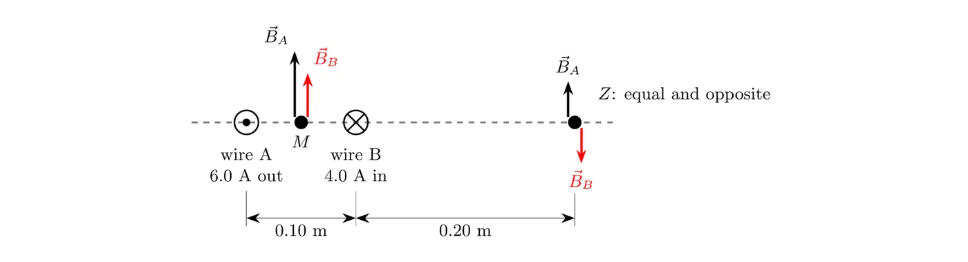
Example. Two long parallel wires are 0.10 m apart. Wire A carries 6.0 A out of the page, and wire B carries 4.0 A into the page. Find the net field at the midpoint M, and find the point on the line through the wires where the field is zero.

At the midpoint (0.050 m from each wire):

B_A = \frac{\mu_0(6.0 \text{ A})}{2\pi(0.050 \text{ m})} = 2.4 \times 10^{-5} \text{ T} \qquad B_B = \frac{\mu_0(4.0 \text{ A})}{2\pi(0.050 \text{ m})} = 1.6 \times 10^{-5} \text{ T}

Directions from the right-hand rule: wire A’s current comes out of the page, so its field circles counterclockwise and points up the page at M. Wire B’s current goes into the page, so its field circles clockwise and also points up the page at M. Same direction, so the sizes add:

B = 4.0 \times 10^{-5}

T, up the page.

Where the field is zero: between the wires, both fields point up, so they can’t cancel. Outside the wires, they point opposite ways. The zero has to be on the side of the weaker current (wire B), where a point can be close to B but farther from A. At a distance

x

from wire A, past wire B:

\frac{\mu_0(6.0)}{2\pi x} = \frac{\mu_0(4.0)}{2\pi(x - 0.10)} \quad\Rightarrow\quad 6.0(x - 0.10) = 4.0x \quad\Rightarrow\quad x = 0.30 \text{ m}

The field is zero 0.30 m from wire A, which is 0.20 m past wire B. Check:

\frac{6.0}{0.30} = \frac{4.0}{0.20} = 20

A/m, so the two fields match.

Cylinders work the same way. A coaxial cable has a central wire carrying

I

one way and a thin outer conducting shell carrying

I

back the other way. A circular Amperian loop between them encloses only the central wire, so

B = \frac{\mu_0 I}{2\pi r}

there. A loop outside the cable encloses

I - I = 0

, so the field outside is zero: the two fields cancel. That’s why a coaxial cable doesn’t make a magnetic field around itself.

Choosing an Amperian Loop

The power of Ampère’s Law comes from picking the right loop to exploit the symmetry.

Guidelines for Choosing Loops

Match the symmetry of the problem.

Cylindrical symmetry means circular loops.

Planar symmetry means rectangular loops.

A solenoid means a rectangular loop with one side inside and one outside.

Make $\vec{B}$ parallel or perpendicular to $d\vec{\ell}$ .

Parallel: $\vec{B} \cdot d\vec{\ell} = B \, d\ell$ , so it contributes fully.

Perpendicular: $\vec{B} \cdot d\vec{\ell} = 0$ , so it contributes nothing.

Choose paths where $B$ is constant.

That makes the integral $\oint B \, d\ell = B \oint d\ell$ easy to evaluate.

Make calculating $I_{enclosed}$ straightforward.

Use symmetry to figure out what current passes through the loop.

When Ampère’s Law is most useful: - High symmetry (infinite wires, solenoids, toroids). - Uniform current distributions. - When you need the field, not just qualitative behavior.

When to use Biot-Savart instead: - Low-symmetry situations. - Finite-length wires. - Arbitrary current configurations.

Maxwell’s Equations: The Complete Set

With the Ampère-Maxwell Law, we now have all four of Maxwell’s equations, which completely describe every electromagnetic phenomenon.

The Four Maxwell’s Equations

1. Gauss’s Law (Electricity):

\oint \vec{E} \cdot d\vec{A} = \frac{Q_{enclosed}}{\epsilon_0}

2. Gauss’s Law (Magnetism):

\oint \vec{B} \cdot d\vec{A} = 0

3. Faraday’s Law:

\oint \vec{E} \cdot d\vec{\ell} = -\frac{d\Phi_B}{dt}

4. Ampère-Maxwell Law:

\oint \vec{B} \cdot d\vec{\ell} = \mu_0 I_{enclosed} + \mu_0\epsilon_0\frac{d\Phi_E}{dt}

Together, these equations: - Unify electricity and magnetism. - Predict electromagnetic waves. - Explain light as electromagnetic radiation. - Form the foundation of classical electrodynamics.

Summary of Key Formulas

Ampère’s Law

\oint \vec{B} \cdot d\vec{\ell} = \mu_0 I_{enclosed}

Common Magnetic Field Results

Configuration	Magnetic Field	Notes
Long straight wire	$B = \frac{\mu_0 I}{2\pi r}$	At distance $r$ from the wire
Solenoid (inside)	$B = \mu_0 n I$	$n$ = turns per length
Solenoid (outside)	$B \approx 0$	Ideally zero for an infinite solenoid
Cylinder (inside, r < R)	$B = \frac{\mu_0 I r}{2\pi R^2}$	Linear in $r$
Cylinder (outside, r > R)	$B = \frac{\mu_0 I}{2\pi r}$	Same as a thin wire

Common Mistakes

Choosing the wrong Amperian loop. The loop has to exploit the symmetry. For a straight wire, use a circular loop, not a square one. For a solenoid, use a rectangular loop with one side inside and one outside, not a circular loop.

Forgetting to count only the enclosed current. Ampère’s Law uses $I_{enclosed}$ , not the total current in the system. When the loop sits inside a conductor with distributed current, you have to calculate what fraction of the current passes through the loop area.

Assuming symmetry where there isn’t any. Ampère’s Law is only practically useful when there’s enough symmetry to pull $B$ out of the integral. For finite wires or complex geometries, you have to use Biot-Savart instead.

Confusing the line integral with the surface integral. Gauss’s Law uses a surface integral ( $\oint \vec{E} \cdot d\vec{A}$ ) over a closed surface. Ampère’s Law uses a line integral ( $\oint \vec{B} \cdot d\vec{\ell}$ ) around a closed path. Don’t mix up the notation or the geometry.

Mixing up the inside and outside formulas. For a cylinder, the field inside grows linearly from zero at the center ( $B \propto r$ ). Outside, it drops as inverse distance ( $B \propto 1/r$ ). Students often wrongly think the field is strongest at the center, or they use the same formula for both regions.

Back Next