

4.7 - The Loanable Funds Market
Setup
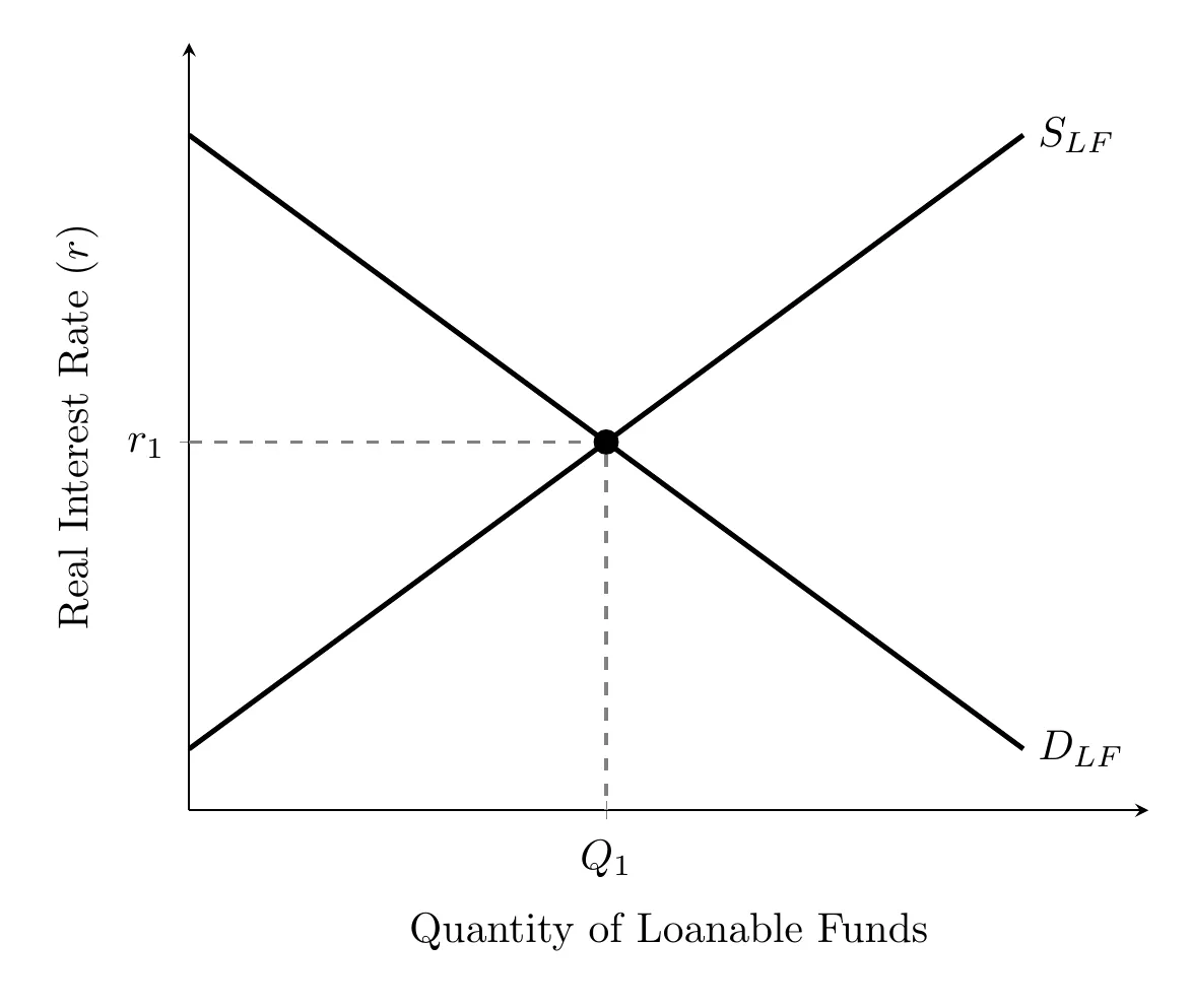
The loanable funds market brings together every borrower and every saver in the economy. It’s not the same thing as “money.” The axes are: real interest rate on the y-axis, quantity of loanable funds on the x-axis. We use the real rate here because that’s what actually guides borrowing and lending decisions.
Supply of Loanable Funds (Savers)
The supply curve represents savers and lenders. Economists treat saving and lending as basically the same activity, with banks just acting as the middleman. The curve slopes upward because savers want a higher return for lending out their money.
In a closed economy, national savings equals public savings plus private savings:
- Private savings = disposable income − consumption
- Public savings = tax revenue − government spending
In an open economy, savings supply also includes net capital inflows (foreign savings coming in). And overall, total savings equals total investment spending, known as the savings-investment identity.
For example, if national savings is $800 billion and $200 billion of foreign savings flows in, the economy can fund $1,000 billion of investment. In a closed economy, net capital inflow is zero, so investment just equals national savings.
Demand for Loanable Funds (Borrowers)
The demand curve represents private borrowers, mostly businesses borrowing to invest (plus households borrowing for things like new homes). It slopes downward since borrowers prefer paying less to borrow. In these notes, government borrowing shows up on the supply side instead, as negative public savings (see the shifters below).
Equilibrium
The loanable funds market is in equilibrium at the real interest rate where the quantity of loanable funds supplied equals the quantity demanded. That’s where the curves cross, at in the graph at the top of the page. At any other rate, the rate adjusts:
- Rate above equilibrium (surplus of loanable funds): savers want to lend more than borrowers want to borrow. Lenders compete for borrowers by offering lower rates, so the real interest rate falls back to equilibrium.
- Rate below equilibrium (shortage of loanable funds): borrowers want more funds than savers are willing to lend. Borrowers compete by offering higher rates, so the real interest rate rises back to equilibrium.
Shifters
Demand shifters:
- Business optimism/pessimism: optimism about future opportunities increases demand for loans (shifts right, raising rates); pessimism decreases it.
- Government investment policy: an investment tax credit lowers the cost of new investment projects, so firms want to borrow more at every interest rate, shifting demand right. Removing it or raising taxes on business investment shifts demand left.
Supply shifters:
- National income/Real GDP: higher income means more private savings, shifting supply right and pushing rates down. Lower income shifts supply left.
- Saving behavior: if households decide to save a bigger share of their income (say, for retirement, or because they’re worried about the future), supply shifts right and pushes rates down. If they save less, supply shifts left.
- Budget deficits: a bigger government deficit reduces public savings, shifting supply left and pushing rates up. This means expansionary fiscal policy (which usually widens the deficit) tends to raise real rates. A surplus shifts supply right.
- Net capital inflows: more foreign saving flowing into the U.S. shifts supply right; more Americans saving abroad shifts it left.
How shifts change the equilibrium: every shift changes both the real interest rate and the quantity of loanable funds.
- Demand increases: the real interest rate and the quantity both rise.
- Demand decreases: the real interest rate and the quantity both fall.
- Supply increases: the real interest rate falls and the quantity rises.
- Supply decreases: the real interest rate rises and the quantity falls.
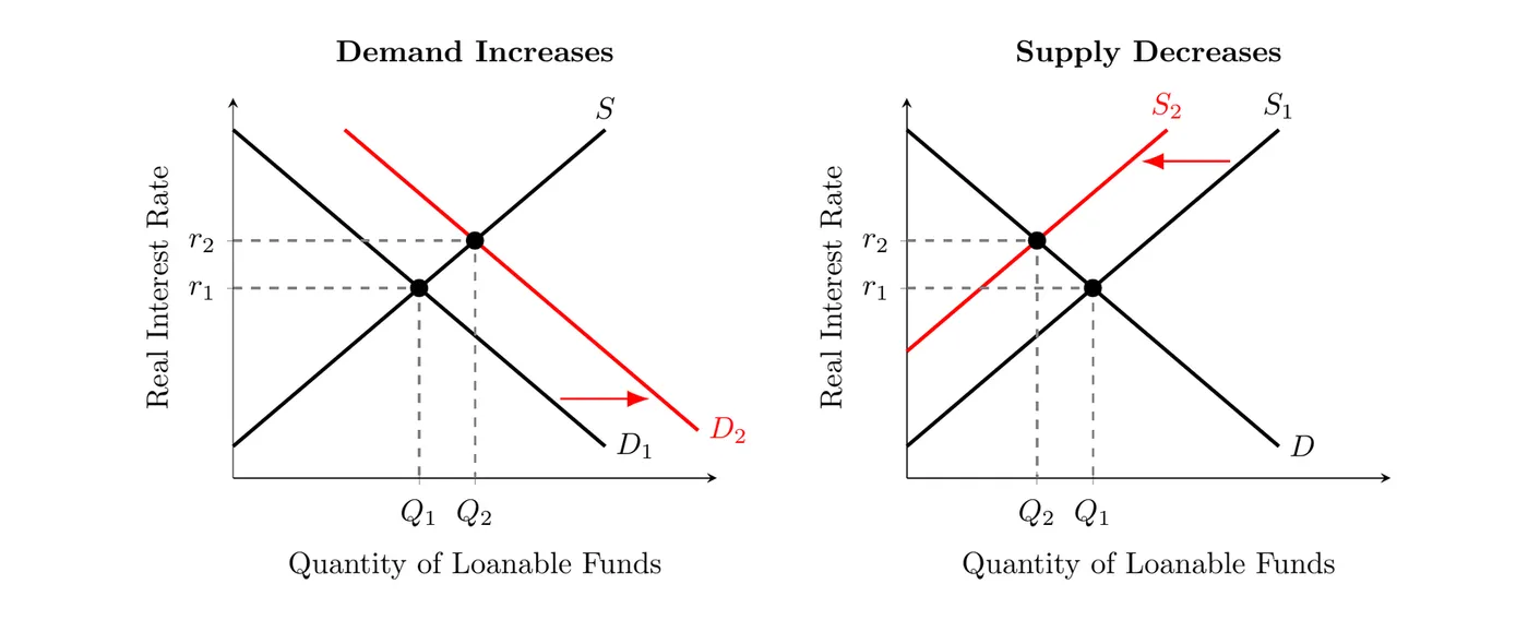
In the left graph, an investment tax credit increases the demand for loanable funds from to , so the real interest rate rises from to and the quantity of loanable funds rises from to . In the right graph, a bigger budget deficit cuts public savings, so supply decreases from to . The real interest rate again rises from to , but the quantity falls from to .
Two ways to show a deficit: these notes show a budget deficit on the supply side, as less public saving, so supply shifts left (the right graph above, and 5.5). Some textbooks and teachers show the same deficit as the government adding to the demand for loanable funds, so demand shifts right instead. The AP exam accepts either graph, and both give the same result: the real interest rate rises and private investment falls, which is crowding out (5.5). Just pick one and stick with it, so you don’t count the deficit twice.
Bottom line: the loanable funds market sets the real interest rate by matching savers (supply) with borrowers (demand). A key takeaway: when the government runs a big budget deficit, it shrinks the supply of savings in the economy, pushing the real interest rate up.