7.3 - Sketching Slope Fields

What is a Slope Field?

A slope field, also called a direction field, is a visual representation of a differential equation. It shows the slope of solution curves at various points in the coordinate plane using small line segments, called hash marks.

Each hash mark represents the slope value you get when you plug that point’s coordinates into the differential equation. All those marks together show the behavior of every possible solution to the differential equation, which is the general solution with all possible values of

C

A slope field only shows hash marks at a finite set of points, usually the points with integer coordinates in a small window. The differential equation gives a slope at every point, but you can’t draw infinitely many marks, so you sample a grid and let your eye fill in the gaps.

Example: Basic Slope Field

Consider the differential equation:

\frac{dy}{dx} = 3x

To find the slope at any point

(x, y)

, substitute the

x

-coordinate. At the point

(-2, 1)

\frac{dy}{dx} = 3(-2) = -6

So we draw a small line segment with slope

-6

at that point.

The general solution is:

y = \int 3x\,dx = \frac{3x^2}{2} + C

The slope field represents all the possible parabolas of the form

y = \frac{3x^2}{2} + C

for any constant

C

Creating a Slope Field: Step by Step

Method 1: Point-by-Point Substitution

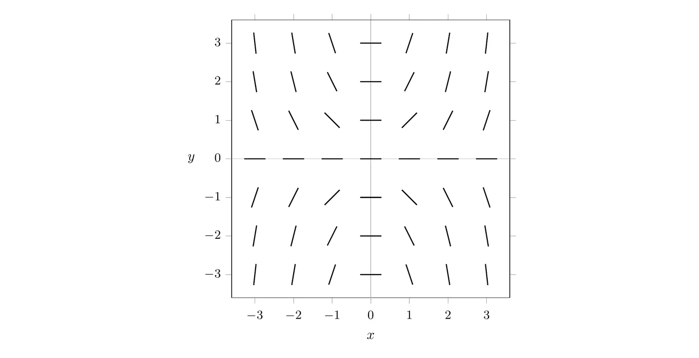
Example: Sketch a slope field for

\frac{dy}{dx} = xy

Step 1: Identify the easy points

Start with the points where the slope is zero or easy to calculate.

Slope of 0 happens when

x = 0

y = 0

: - Draw horizontal hash marks all along the

x

-axis, where

y = 0

- Draw horizontal hash marks all along the

y

-axis, where

x = 0

Step 2: Calculate slopes at specific points

Point	Calculation	Slope
$(1, 1)$	$1 \cdot 1$	$1$
$(2, 1)$	$2 \cdot 1$	$2$
$(-1, 2)$	$(-1) \cdot 2$	$-2$
$(2, 2)$	$2 \cdot 2$	$4$
$(-2, -1)$	$(-2) \cdot (-1)$	$2$
$(1, -2)$	$1 \cdot (-2)$	$-2$

Step 3: Draw the hash marks

At each point, draw a small line segment with the slope you calculated. They don’t have to be perfectly precise, so just eyeball the angle.

Method 2: Organized Chart

For more complicated differential equations, make a systematic chart.

Example: Sketch a slope field for

\frac{dy}{dx} = x + 3

$x$	$y$	$\frac{dy}{dx}$
$-2$	$2$	$1$
$-2$	$1$	$1$
$-2$	$0$	$1$
$-1$	$2$	$2$
$-1$	$1$	$2$
$-1$	$0$	$2$
$0$	$2$	$3$
$0$	$1$	$3$
$0$	$0$	$3$
$1$	$2$	$4$
$1$	$1$	$4$

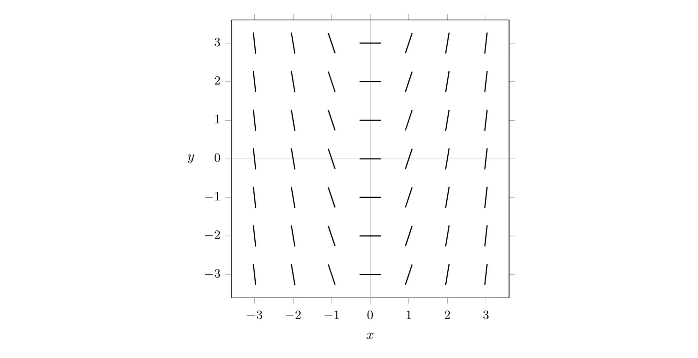
Notice that for this equation, every point with the same

x

-coordinate has the same slope, since the equation doesn’t depend on

y

. That means the hash marks form vertical columns with identical slopes.

Visualizing Solution Curves

Conceptual tip: think of the hash marks as currents in a river. If you dropped a leaf at any point, it would flow along the direction the hash marks point, tracing out a solution curve.

The hash marks show: - Where curves increase, meaning positive slopes - Where curves decrease, meaning negative slopes - Local maxima, where horizontal hash marks appear and slopes change from positive to negative - Local minima, where horizontal hash marks appear and slopes change from negative to positive

You can read concavity too. Follow a curve to the right: if the hash marks get steeper (the slopes increase), the curve is concave up. If the slopes decrease, it’s concave down.

To check concavity exactly, find

\frac{d^2y}{dx^2}

by differentiating the differential equation with respect to

x

. Since

y

is a function of

x

, every

y

term gets a

\frac{dy}{dx}

(implicit differentiation). For

\frac{dy}{dx} = x + y

\frac{d^2y}{dx^2} = 1 + \frac{dy}{dx} = 1 + x + y

(1, 1)

\frac{dy}{dx} = 2

and

\frac{d^2y}{dx^2} = 1 + 1 + 1 = 3

, so the solution curve through

(1, 1)

is increasing and concave up there.

Finding Tangent Lines Using Slope Fields

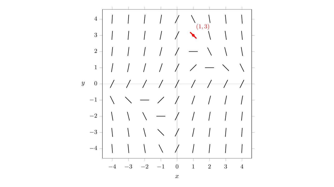
Problem: Given the differential equation

\frac{dy}{dx} = 2 - xy

and its slope field, find the equation of the tangent line at the point

(1, 3)

Step 1: Find the slope

Substitute

(1, 3)

into the differential equation:

\frac{dy}{dx} = 2 - (1)(3) = 2 - 3 = -1

Step 2: Write the tangent line equation

Using point-slope form:

y - 3 = -1(x - 1)

y - 3 = -x + 1

y = -x + 4

The slope field confirms this, since at

(1, 3)

the hash mark should have slope

-1

Matching Slope Fields to Differential Equations

Given a slope field, you can figure out which differential equation it represents by looking at patterns.

Strategy: Look for Key Features

1. Horizontal hash marks (slope = 0)

These show up where the derivative equals zero. Find where the horizontal marks appear.

2. Vertical hash marks (undefined slope)

These show up where the derivative is undefined, meaning division by zero. Look for curves or lines where no hash marks exist, or where vertical marks appear.

3. Symmetry patterns

Check whether the field is symmetric about the axes or about specific lines.

Example Problem

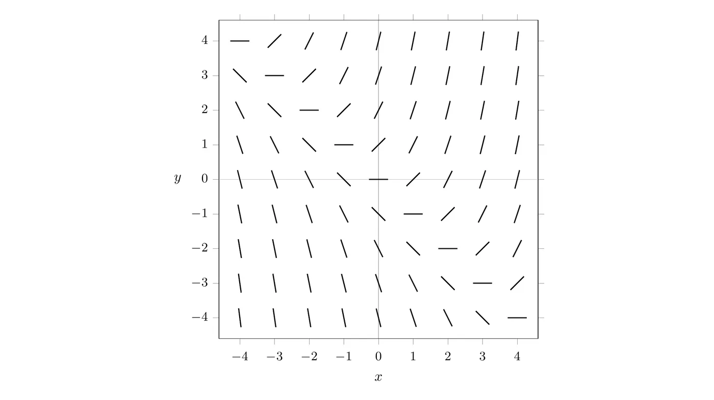
Which differential equation matches this slope field?

(A)

\frac{dy}{dx} = \frac{x}{y}

(B)

\frac{dy}{dx} = x^2 + y^2

(C)

\frac{dy}{dx} = x + y

(D)

\frac{dy}{dx} = \frac{1}{x-y}

Analysis:

Check for horizontal marks. They appear when

y = -x

, along the diagonal.

Test (A) at

x = 2

y = -2

\frac{2}{-2} = -1 \neq 0

✗

Test (B) at

x = 2

y = -2

4 + 4 = 8 \neq 0

✗

Test (C) at

x = 2

y = -2

2 + (-2) = 0

✓

Test (D) at

x = 2

y = -2

\frac{1}{2-(-2)} = \frac{1}{4} \neq 0

✗

Check for vertical marks. Option (D) would have undefined slopes when

x = y

, but the slope field shows no vertical marks, so (D) is out.

Verify with another point. At

(1, 1)

the slope should be positive. Option (C) gives

1 + 1 = 2

✓, which is a positive slope, and that matches the slope field.

Answer: (C)

\frac{dy}{dx} = x + y

Common Slope Field Patterns

Pattern 1: Slopes depend only on $x$

Example:

\frac{dy}{dx} = x - 2

Every point on the same vertical line, meaning the same

x

-value, has an identical slope. The hash marks form vertical columns.

Pattern 2: Slopes depend only on $y$

Example:

\frac{dy}{dx} = y + 1

Every point on the same horizontal line, meaning the same

y

-value, has an identical slope. The hash marks form horizontal rows.

Pattern 3: Slopes depend on both $x$ and $y$

Example:

\frac{dy}{dx} = xy

Slopes vary based on both coordinates, which creates more complex patterns with curved solution paths.

Key Takeaways

Slope field: a visual representation showing the slopes of all the solution curves to a differential equation

Finite set of points: a slope field only shows marks on a grid of points, even though the differential equation gives a slope everywhere

Hash marks: small line segments drawn at each point with slope $= \frac{dy}{dx}$ at that point

General solution: a slope field represents all the possible solutions, meaning all values of $C$

Creating slope fields: substitute coordinates into $\frac{dy}{dx}$ to find the slope at each point

Horizontal marks appear where $\frac{dy}{dx} = 0$ , which points to maxima, minima, or inflection points

Vertical marks appear where $\frac{dy}{dx}$ is undefined, meaning division by zero

Concavity: find $\frac{d^2y}{dx^2}$ by differentiating the differential equation (implicitly), then plug in the point

Tangent lines: use the differential equation to find the slope at a point, then apply point-slope form

Matching strategy: test points, especially where the slope is 0, in each differential equation to find matches

Visualization tip: think of the hash marks as river currents guiding the solution curves

Back Next

7.3 - Sketching Slope Fields

What is a Slope Field?

Example: Basic Slope Field

Creating a Slope Field: Step by Step

Method 1: Point-by-Point Substitution

Method 2: Organized Chart

Visualizing Solution Curves

Finding Tangent Lines Using Slope Fields

Matching Slope Fields to Differential Equations

Strategy: Look for Key Features

Example Problem

Common Slope Field Patterns

Pattern 1: Slopes depend only on xxx

Pattern 2: Slopes depend only on yyy

Pattern 3: Slopes depend on both xxx and yyy

Key Takeaways

Pattern 1: Slopes depend only on $x$

Pattern 2: Slopes depend only on $y$

Pattern 3: Slopes depend on both $x$ and $y$