7.7 - Finding Particular Solutions Using Initial Conditions and Separation of Variables

Introduction to Particular Solutions

In previous lessons we found general solutions to differential equations, meaning solutions with an arbitrary constant

C

in them. Now we’ll use separation of variables together with initial conditions to find particular solutions, which are specific functions with the constant pinned down.

The key difference: we solve for the exact value of

C

using a given point, which gives us one complete solution equation.

A general solution describes infinitely many solutions, one for each value of

C

. But only one particular solution passes through a given point, so one initial condition is enough to pin down the answer.

The Process: Separation of Variables with Initial Conditions

Separate the variables. Get all the $y$ terms (including $dy$ ) on one side and all the $x$ terms (including $dx$ ) on the other

Integrate both sides

Either Option A: solve for $C$ immediately using the initial condition, or Option B: solve for $y$ first, then find $C$

Write the particular solution with the specific value of $C$

Example 1: Basic Separation with Polynomial Terms

Problem: Find the particular solution to

\frac{dy}{dx} = x^2y^2

that passes through

(1, 1)

Step 1: Separate the variables

\frac{dy}{dx} = x^2y^2

Divide both sides by

y^2

and multiply by

dx

y^{-2}\,dy = x^2\,dx

Step 2: Integrate both sides

\int y^{-2}\,dy = \int x^2\,dx

\frac{y^{-1}}{-1} = \frac{x^3}{3} + C

-\frac{1}{y} = \frac{x^3}{3} + C

Step 3: Find $C$ using the initial condition

Substitute

(1, 1)

-\frac{1}{1} = \frac{1^3}{3} + C

-1 = \frac{1}{3} + C

C = -1 - \frac{1}{3} = -\frac{4}{3}

Step 4: Solve for $y$ with the specific constant

-\frac{1}{y} = \frac{x^3}{3} - \frac{4}{3}

Multiply both sides by

-1

\frac{1}{y} = -\frac{x^3}{3} + \frac{4}{3}

Combine the fractions:

\frac{1}{y} = \frac{4 - x^3}{3}

Take the reciprocal:

y = \frac{3}{4 - x^3}

Particular solution:

y = \frac{3}{4 - x^3}

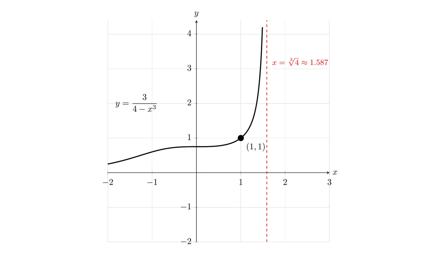
Domain Restrictions

A particular solution has to be differentiable on an interval that contains the initial point. It can’t jump across a spot where it’s undefined.

Here,

y = \frac{3}{4 - x^3}

is undefined where

4 - x^3 = 0

, at

x = \sqrt[3]{4} \approx 1.587

. The initial point has

x = 1

, which is to the left of that asymptote, so the particular solution is only the left piece:

y = \frac{3}{4 - x^3}, \quad x < \sqrt[3]{4}

That’s why the graph above stops at the asymptote. Watch for anything that makes a solution undefined (a zero denominator, a negative number under a square root, the log of zero or a negative number), and keep only the interval that contains the initial

x

-value.

Example 2: Determining the Sign (Plus or Minus)

Problem: Solve

\frac{dy}{dx} = 2xy

with the initial condition

y(2) = 1

Step 1: Separate the variables

\frac{dy}{y} = 2x\,dx

Step 2: Integrate both sides

\int \frac{dy}{y} = \int 2x\,dx

\ln|y| = x^2 + C_1

Optional simplification: multiply both sides by 2 to avoid fractions later:

2\ln|y| = 2x^2 + 2C_1

\ln(y^2) = 2x^2 + C

We can drop the absolute values inside, since

y^2

is always non-negative, and we’re just calling

2C_1

by the name

C

Step 3: Find the constant using $(2, 1)$

\ln(1^2) = 2(2^2) + C

0 = 8 + C

C = -8

Step 4: Solve for $y$

\ln(y^2) = 2x^2 - 8

y^2 = e^{2x^2 - 8}

Take the square root of both sides:

y = \pm e^{x^2 - 4}

Critical decision: which sign do we pick?

Check the initial condition. At

(2, 1)

, the

y

-value is positive, so we need the positive square root.

Particular solution:

y = e^{x^2 - 4}

Understanding the Graph

The implicit form

y^2 = e^{2x^2 - 8}

represents both the positive and the negative square root functions. But the particular solution through

(2, 1)

is only the top half of that curve.

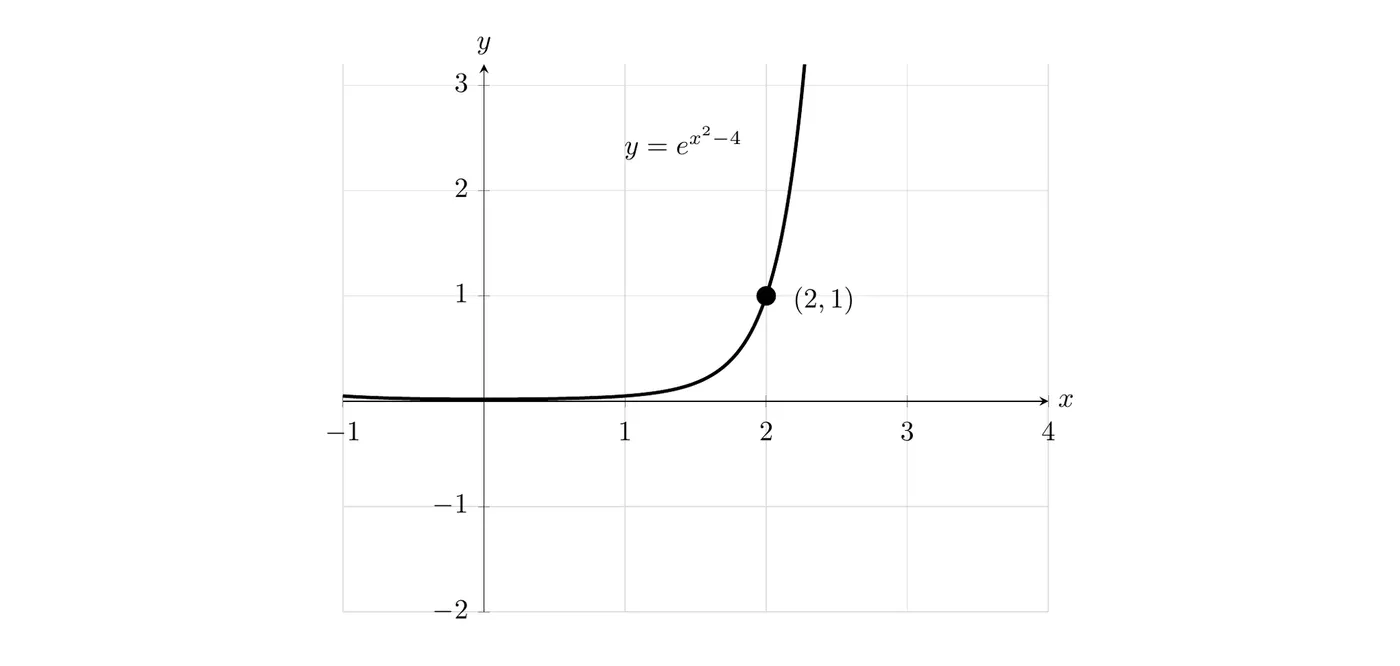
If we’d chosen the negative square root, the solution would be the bottom half, reflected across the

x

-axis.

Example 3: Handling Absolute Values

Problem: Find the particular solution to

\frac{dy}{dx} = (y + 3)e^x

that passes through

(0, -2)

Step 1: Separate the variables

\frac{dy}{y + 3} = e^x\,dx

Step 2: Integrate both sides

\int \frac{dy}{y + 3} = \int e^x\,dx

\ln|y + 3| = e^x + C

Step 3: Find $C$ using $(0, -2)$

\ln|-2 + 3| = e^0 + C

\ln(1) = 1 + C

0 = 1 + C

C = -1

So we have:

\ln|y + 3| = e^x - 1

Step 4: Exponentiate both sides

e^{\ln|y + 3|} = e^{e^x - 1}

|y + 3| = e^{e^x - 1}

Important: when you remove absolute values, include the

\pm

y + 3 = \pm e^{e^x - 1}

y = \pm e^{e^x - 1} - 3

Step 5: Determine the correct sign

Substitute

x = 0

to see which sign gives

y = -2

y = \pm e^{e^0 - 1} - 3

y = \pm e^{1-1} - 3

y = \pm e^0 - 3

y = \pm 1 - 3

For

y = -2

, we need

\pm 1 - 3 = -2

, which means

\pm 1 = 1

. So use the positive sign.

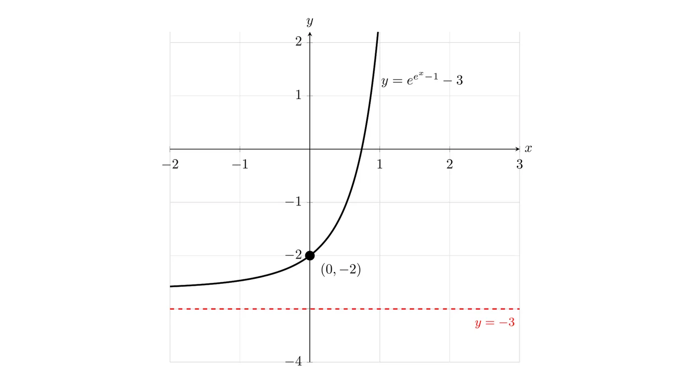
Particular solution:

y = e^{e^x - 1} - 3

When to Choose Plus vs. Minus

After taking a square root or removing absolute values, you’ll often be left with a

\pm

. Here’s how to figure out which one is right.

Method 1: Test the Initial Condition

Substitute the given point into both versions and see which one satisfies the condition.

Method 2: Use the Slope Field, If You Have One

Sketch or visualize where the solution curve should be. Does it lie above or below the

x

-axis? Is it the upper or lower branch of the curve?

Method 3: Consider the Physical Context

Sometimes the context of the problem, like population growth or temperature, tells you whether the values should be positive or negative.

Why Absolute Values Create Plus/Minus

Review from algebra: when solving

|x - 2| = 5

, you get two equations:

x - 2 = 5 \quad \text{or} \quad x - 2 = -5

x = 7 \quad \text{or} \quad x = -3

Both solutions are valid, since

|7 - 2| = 5

and

|-3 - 2| = 5

In differential equations: when we have

\ln|y + 3| = e^x - 1

and exponentiate:

|y + 3| = e^{e^x - 1}

The absolute value means:

y + 3 = e^{e^x - 1} \quad \text{or} \quad y + 3 = -e^{e^x - 1}

which leads to:

y = e^{e^x - 1} - 3 \quad \text{or} \quad y = -e^{e^x - 1} - 3

Particular Solutions as Accumulation Functions

When the differential equation only involves

x

, like

\frac{dy}{dx} = f(x)

, you can write the particular solution through

(a, y_0)

directly as an accumulation function:

F(x) = y_0 + \int_a^x f(t)\,dt

Why it works:

By the Fundamental Theorem of Calculus, $F'(x) = f(x)$ , so $F$ solves the differential equation

At $x = a$ , the integral runs from $a$ to $a$ , so it equals $0$ and $F(a) = y_0$ . So $F$ passes through the initial point

This is the same idea as an accumulation function from Unit 6: start at

y_0

, then add up the change from

a

x

Example: Find the particular solution to

\frac{dy}{dx} = e^{-x^2}

with

y(1) = 4

, and approximate

y(2)

e^{-x^2}

has no antiderivative made of basic functions, so integrating and solving for

C

gets stuck. The accumulation form still works:

y = 4 + \int_1^x e^{-t^2}\,dt

Then use a calculator for the definite integral:

y(2) = 4 + \int_1^2 e^{-t^2}\,dt \approx 4 + 0.135 = 4.135

Strategic Tips for Solving

Tip 1: Simplify Before Finding $C$

Sometimes multiplying or dividing by a constant early makes the algebra cleaner.

Example: if you have

\frac{y^2}{2} = x^2 + C_1

, multiply by 2 to get

y^2 = 2x^2 + C

, where

C = 2C_1

. That way you avoid working with fractions when you substitute the initial condition.

Tip 2: When to Find $C$

Find $C$ early if the equation is complicated to solve for $y$

Solve for $y$ first if finding $C$ will be easier once $y$ is isolated

Both approaches work, so pick whichever looks simpler.

Tip 3: Keep Track of Constants

When you multiply or divide the whole equation by a number, your constant changes. You might see something like:

C_1 \rightarrow C_2 = 2C_1 \rightarrow C_3 = C_2 + 5

Don’t worry about subscripts unless you need them for clarity. Just remember the constant changes, and it has to be recalculated if you transformed the equation before finding it.

Common Mistakes to Avoid

❌ Forgetting the $\pm$ when taking square roots or removing absolute values. Always write the $\pm$ , then use the initial condition to pick the sign

❌ Assuming a negative $y$ -value means you use the negative sign. Check by substitution, since that isn’t automatic

❌ Dropping absolute values without considering both cases. When $\ln|f(y)| = g(x)$ , exponentiating gives $|f(y)| = e^{g(x)}$ , which means $f(y) = \pm e^{g(x)}$

❌ Not checking your answer. Always verify that the final answer satisfies both the differential equation and the initial condition

Summary of the Process

Given

\frac{dy}{dx} = f(x, y)

with the initial condition

(x_0, y_0)

Separate the variables: $g(y)\,dy = h(x)\,dx$

Integrate: $\int g(y)\,dy = \int h(x)\,dx + C$

Find $C$ : substitute $(x_0, y_0)$ and solve

Solve for $y$ : isolate $y$ , watching for the $\pm$ when you take roots or exponentiate

Determine the sign: use the initial condition to pick the correct one if you need to

Write the particular solution

Key Takeaways

Particular solution: a specific function satisfying both the differential equation and an initial condition

One point, one solution: a general solution is a whole family, but only one particular solution passes through a given point

Two approaches: find $C$ before or after solving for $y$ . Both work, so choose strategically

Taking square roots: always include the $\pm$ , then use the initial condition to determine the sign

Removing absolute values: exponentiating $\ln|f(y)| = g(x)$ gives $f(y) = \pm e^{g(x)}$

Choosing the sign: substitute the initial condition into both possibilities and see which one works

Slope fields help. Visualizing the solution curve can make it clear which sign is right

Constants transform. When you multiply or divide the equation, the constant changes, but it’s still just “some constant”

Verification: always check your final answer by substituting the initial condition

Implicit vs. explicit: the equation with the $\pm$ represents multiple curves, and the particular solution is just one of them

Domain restrictions: the particular solution only lives on the interval that contains the initial point, so stop at asymptotes and other places where it’s undefined

Accumulation form: the solution to $\frac{dy}{dx} = f(x)$ with $y(a) = y_0$ is $y = y_0 + \int_a^x f(t)\,dt$

Back Next

7.7 - Finding Particular Solutions Using Initial Conditions and Separation of Variables

Introduction to Particular Solutions

The Process: Separation of Variables with Initial Conditions

Example 1: Basic Separation with Polynomial Terms

Domain Restrictions

Example 2: Determining the Sign (Plus or Minus)

Understanding the Graph

Example 3: Handling Absolute Values

When to Choose Plus vs. Minus

Method 1: Test the Initial Condition

Method 2: Use the Slope Field, If You Have One

Method 3: Consider the Physical Context

Why Absolute Values Create Plus/Minus

Particular Solutions as Accumulation Functions

Strategic Tips for Solving

Tip 1: Simplify Before Finding CCC

Tip 2: When to Find CCC

Tip 3: Keep Track of Constants

Common Mistakes to Avoid

Summary of the Process

Key Takeaways

Tip 1: Simplify Before Finding $C$

Tip 2: When to Find $C$