7.5 - Approximating Solutions Using Euler's Method (BC ONLY)

Note: this is a BC Calculus topic only, and it isn’t required for AB Calculus.

Introduction to Euler’s Method

Euler’s Method, pronounced “OY-ler,” is a technique for finding an approximate solution to a differential equation when you can’t easily find an exact one. It was developed by the Swiss mathematician Leonhard Euler.

The key idea: instead of finding the actual solution curve, we build a series of small tangent line segments that approximate it. Each segment uses the slope given by the differential equation.

The Concept: Tangent Line Approximations

Consider a differential equation

\frac{dy}{dx} = f(x, y)

with an initial condition, meaning a point the solution passes through.

Starting at the known point, we:

Calculate the slope using the differential equation

Move a small distance, the step size, along the tangent line

Find our new point

Repeat

Each tangent line segment approximates a small piece of the actual solution curve.

Visual Representation

Example: For

\frac{dy}{dx} = 1 + y

passing through

(0, 0)

with step size

\Delta x = 0.5

7.5 - Approximating Solutions Using Euler's Method (BC ONLY)

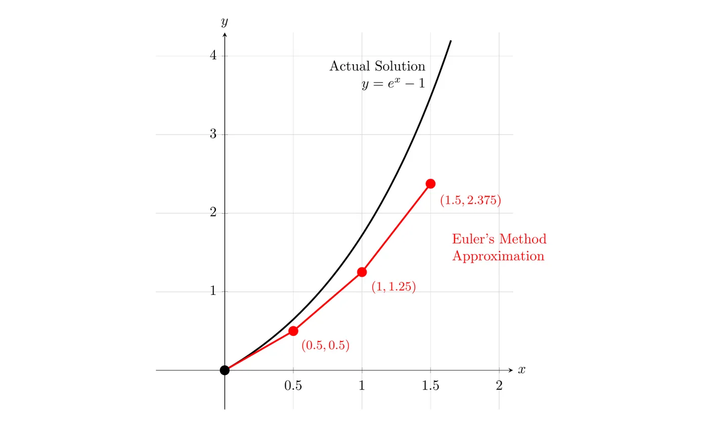
Observation: the Euler approximation stays close to the actual curve at first, but it drifts further away as you keep going. Smaller step sizes give more accurate approximations.

The Step Size Formula

The step size, written

\Delta x

, is the horizontal distance between consecutive points.

If you need to approximate

f(b)

starting from

f(a)

using

n

steps:

\Delta x = \frac{b - a}{n}

Example: to approximate

f(3)

starting from

f(1)

using 4 steps:

\Delta x = \frac{3 - 1}{4} = \frac{2}{4} = 0.5

So each step moves

0.5

units in the

x

-direction.

The Euler’s Method Formula

This is the key formula to memorize:

\boxed{y_{\text{new}} = y_{\text{old}} + \frac{dy}{dx} \cdot \Delta x}

Or equivalently:

\boxed{y_{\text{new}} = y_{\text{old}} + y' \cdot \Delta x}

What each term means: -

y_{\text{new}}

: the

y

-coordinate of the next point -

y_{\text{old}}

: the

y

-coordinate of the current point -

\frac{dy}{dx}

y'

: the slope from the differential equation, evaluated at the current point -

\Delta x

: the step size, which stays constant throughout

Connection to point-slope form: this formula comes straight from the point-slope form of a line:

y - y_1 = m(x - x_1)

Solving for

y

when

x = x_1 + \Delta x

y = y_1 + m \cdot \Delta x

Organizing Your Work: The Euler’s Method Table

The best way to keep Euler’s method calculations organized is with a table:

x

y

\frac{dy}{dx}

y_{\text{new}} = y + \frac{dy}{dx} \cdot \Delta x

Process for each row:

Write the current $x$ and $y$ values

Calculate $\frac{dy}{dx}$ by substituting $x$ and $y$ into the differential equation

Calculate $y_{\text{new}}$ using the Euler formula

Move to the next row, where the new $x$ = old $x$ + $\Delta x$ , and $y$ = $y_{\text{new}}$ from the previous row

Example 1: Two-Step Approximation

Problem: Given

\frac{dy}{dx} = x - y

with

y(0) = 2

, use Euler’s method with

\Delta x = 0.5

to approximate

y(1)

Step 1: Determine the number of steps

From

x = 0

x = 1

with

\Delta x = 0.5

\text{Number of steps} = \frac{1 - 0}{0.5} = 2 \text{ steps}

Step 2: Set up the table

$x$	$y$	$\frac{dy}{dx} = x - y$	$y_{\text{new}} = y + \frac{dy}{dx}(0.5)$
$0$	$2$	$0 - 2 = -2$	$2 + (-2)(0.5) = 1$
$0.5$	$1$	$0.5 - 1 = -0.5$	$1 + (-0.5)(0.5) = 0.75$
$1$	$0.75$

Step 3: State the answer

y(1) \approx 0.75

Example 2: Three-Step Approximation

Problem: Given

\frac{dy}{dx} = xy

with

y(1) = 2

, use Euler’s method with step size

0.4

to approximate

y(2.2)

Step 1: Calculate the step size information

From

x = 1

x = 2.2

, the distance is

2.2 - 1 = 1.2

With

\Delta x = 0.4

\text{Number of steps} = \frac{1.2}{0.4} = 3 \text{ steps}

Step 2: Create the Euler’s method table

$x$	$y$	$\frac{dy}{dx} = xy$	$y_{\text{new}} = y + (xy)(0.4)$
$1$	$2$	$(1)(2) = 2$	$2 + 2(0.4) = 2.8$
$1.4$	$2.8$	$(1.4)(2.8) = 3.92$	$2.8 + 3.92(0.4) = 4.368$
$1.8$	$4.368$	$(1.8)(4.368) = 7.8624$	$4.368 + 7.8624(0.4) = 7.51296$
$2.2$	$7.51296$

Step 3: State the answer

y(2.2) \approx 7.513

Important: don’t round the intermediate values. Keep all the decimal places until the final answer so rounding errors don’t pile up.

Example 3: Multi-Step Problem with Five Steps

Problem: Given

\frac{dy}{dx} = 3x

with

f(2) = 5

, use Euler’s method with 5 steps to approximate

f(3)

Step 1: Calculate the step size

\Delta x = \frac{3 - 2}{5} = \frac{1}{5} = 0.2

Step 2: Build the table systematically

$x$	$y$	$\frac{dy}{dx} = 3x$	$y_{\text{new}} = y + (3x)(0.2)$
$2$	$5$	$3(2) = 6$	$5 + 6(0.2) = 6.2$
$2.2$	$6.2$	$3(2.2) = 6.6$	$6.2 + 6.6(0.2) = 7.52$
$2.4$	$7.52$	$3(2.4) = 7.2$	$7.52 + 7.2(0.2) = 8.96$
$2.6$	$8.96$	$3(2.6) = 7.8$	$8.96 + 7.8(0.2) = 10.52$
$2.8$	$10.52$	$3(2.8) = 8.4$	$10.52 + 8.4(0.2) = 12.2$
$3$	$12.2$

Answer:

f(3) \approx 12.2

Accuracy Considerations

Factors Affecting Accuracy

Step size: smaller $\Delta x$ means a more accurate approximation

Number of steps: more steps means you get closer to the actual solution

Behavior of the function: rapidly changing functions need smaller steps

Error Accumulation

Every step introduces a small error, because you’re using a straight line to approximate a curve. Those errors accumulate over multiple steps, so:

Euler’s method is most accurate near the starting point

Accuracy gets worse the further you move from the initial condition

The approximation typically underestimates or overestimates consistently, based on concavity

Overestimate or Underestimate?

Euler’s method walks along tangent lines, so the shape of the solution curve tells you which way it’s off:

Concave up ( $\frac{d^2y}{dx^2} > 0$ ): tangent lines sit below the curve, so Euler’s method gives an underestimate

Concave down ( $\frac{d^2y}{dx^2} < 0$ ): tangent lines sit above the curve, so Euler’s method gives an overestimate

To find

\frac{d^2y}{dx^2}

, differentiate the differential equation (implicitly, since

y

depends on

x

). The concavity has to hold over the whole interval you step across, not just at the starting point.

Example: In the Visual Representation example above,

\frac{dy}{dx} = 1 + y

with

y(0) = 0

. Then

\frac{d^2y}{dx^2} = \frac{dy}{dx} = 1 + y

The solution starts at

y = 0

with a positive slope and keeps increasing, so

y \geq 0

and

\frac{d^2y}{dx^2} = 1 + y > 0

the whole way. The curve is concave up, so Euler’s method underestimates. That matches the graph: at

x = 1.5

, Euler’s method gives

2.375

, but the actual value is

e^{1.5} - 1 \approx 3.482

Common Mistakes to Avoid

❌ Rounding too early. Keep all the decimal places during the calculations, and only round the final answer

❌ Forgetting to multiply by $\Delta x$ . The formula is $y_{\text{new}} = y + y' \cdot \Delta x$ , not just $y + y'$

❌ Using the wrong $x$ or $y$ value. Always use the current point’s coordinates to calculate the slope

❌ Miscounting steps. Double-check that $\Delta x = \frac{b-a}{n}$ was calculated correctly

❌ Copying errors. When you move to the next row, make sure $y_{\text{new}}$ from the previous row becomes the new $y$

Step-by-Step Process Summary

Given: a differential equation

\frac{dy}{dx} = f(x, y)

, an initial condition

(x_0, y_0)

, and either a step size

\Delta x

or a number of steps

n

Calculate the step size if you need to: $\Delta x = \frac{x_{\text{final}} - x_0}{n}$

Set up the table with columns for $x$ , $y$ , $\frac{dy}{dx}$ , and $y_{\text{new}}$

Fill in the initial values. The first row has $x_0$ and $y_0$

For each row:

Calculate $\frac{dy}{dx}$ using the differential equation

Calculate $y_{\text{new}} = y + \frac{dy}{dx} \cdot \Delta x$

Next row: $x_{\text{new}} = x + \Delta x$ , and $y$ = $y_{\text{new}}$ from the previous row

Continue until you reach the $x$ -value you want

State the answer. The final $y$ -value is your approximation

Key Takeaways

Euler’s Method: an approximation technique using tangent line segments to estimate solutions to differential equations

Step size formula: $\Delta x = \frac{b - a}{n}$ , where $n$ is the number of steps

Core formula: $y_{\text{new}} = y_{\text{old}} + \frac{dy}{dx} \cdot \Delta x$

Table organization: use columns for $x$ , $y$ , $\frac{dy}{dx}$ , and $y_{\text{new}}$ to stay organized

Accuracy: smaller step sizes give more accurate approximations, but they take more calculations

Over or under: if the solution is concave up, Euler’s method underestimates; if it’s concave down, Euler’s method overestimates

Calculator use: keep all the decimal places in the intermediate steps, and don’t round until the final answer

BC Calculus only. This topic shows up on the BC exam, not the AB exam

Each step uses the current point’s coordinates to find the slope, then moves along the tangent line by $\Delta x$

Back Next