5.2 - Correlation

Overview

A scatterplot shows an association, and the correlation coefficient

r

puts a number on it. It measures the direction and strength of a linear association between two quantitative variables. This topic covers what

r

tells you and two traps students fall into: a value of

r

near 1 or

-1

doesn't prove a line fits, and correlation doesn't prove causation.

What $r$ measures

The correlation coefficient,

r

, summarizes the strength and direction of the linear association between two quantitative variables. Its key properties:

$r$ is always between $-1$ and $1$ , inclusive: $-1 \le r \le 1$ .

The sign gives the direction. A negative $r$ means a negative association, and a positive $r$ means a positive association.

$r$ is unit-free. It has no units, and changing the units of either variable (inches to centimeters, dollars to thousands of dollars) doesn't change it.

$r$ only describes linear association, and only between quantitative variables. For categorical variables, say "association," not "correlation."

Switching which variable is $x$ and which is $y$ doesn't change $r$ .

You'll find

r

with technology: on a TI-84, LinReg(a+bx) reports it once diagnostics are on (Topic 5.5 has the steps).

Why the sign works

You won't compute

r

by hand, and this formula isn't on the AP formula sheet, but it shows where

r

comes from. It averages the products of the

z

-scores:

r = \frac{1}{n - 1}\sum z_x z_y

A point to the right of

\bar{x}

has

z_x > 0

, and a point above

\bar{y}

has

z_y > 0

. So points in the upper right and lower left of

(\bar{x}, \bar{y})

add positive products, and points in the upper left and lower right add negative products. In the figure, each label shows the signs of

(z_x)(z_y)

in that region.

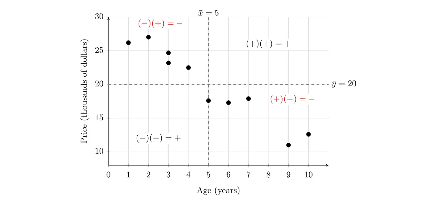
For the used cars from Topic 5.1, nine of the ten points sit in the two negative regions, and the 5-year-old car sits right on the line

x = \bar{x}

(its product is 0). The products add up to a negative number, so

r

is negative. This is also why

r

is unit-free:

z

-scores have no units.

How strong is it?

The strength of the linear association depends on how close

r

is to

-1

1

$r = 1$ or $r = -1$ : a perfect linear association. Every point lies exactly on a line.

$r$ close to $1$ or $-1$ : a strong linear association.

$r$ close to 0: a weak linear association.

$r = 0$ : no linear association. That's not the same as no association at all. There could still be a strong curved pattern.

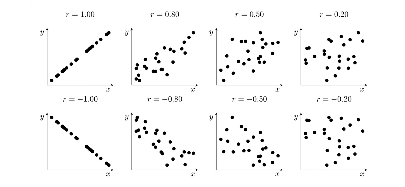
Strength and direction are separate.

r = -0.90

is a stronger association than

r = 0.60

, because

-0.90

is closer to

-1

than

0.60

is to

1

. There are no official cutoffs for the words, but this rough guide works on the exam if you also look at the plot:

Value of $\|r\|$	Usual description
0.8 to 1	strong
0.5 to 0.8	moderate
0 to 0.5	weak

Interpreting $r$ in context

Template: "The correlation of

r =

___ indicates a [strength], [direction] linear association between [explanatory variable] and [response variable]."

Example 1: Interpreting $r$ for the used cars

For the 10 used cars from Topic 5.1, the TI-84 gives

r = -0.963

for age and price. Interpret this value.

Answer:

r = -0.963

indicates a strong, negative linear association between age and listed price for these cars: older cars tend to have lower prices. It's strong because

-0.963

is close to

-1

, and negative because

r < 0

Example 2: Changing units

Suppose the ages were recorded in months and the prices in dollars instead. What is the correlation now?

Answer: still

r = -0.963

. Multiplying every age by 12 and every price by 1,000 changes the numbers on the axes, but not the pattern of the points. Because

r

is unit-free, it doesn't change.

A strong $r$ doesn't mean a line fits

A correlation close to

-1

1

does not necessarily mean a linear model is appropriate.

r

measures how tightly the points cluster around a straight line, and a curved pattern that keeps rising can still give a value close to 1.

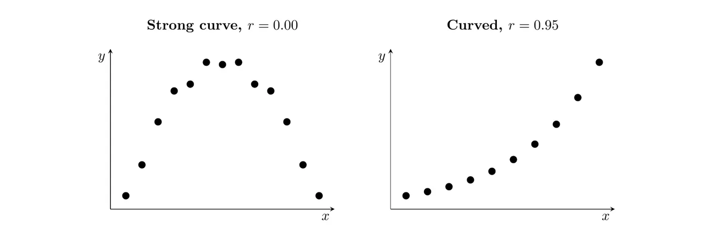
Left: a strong curved pattern with $r = 0.00$ . The rising half and the falling half cancel out, so there's no linear association even though $y$ clearly depends on $x$ .

Right: $r = 0.95$ , but the points clearly bend upward. A line would sit too high in the middle and too low at the ends.

So always look at the scatterplot (and, from Topic 5.4, the residual plot) before you trust

r

or fit a line.

r

is also not resistant: one point that doesn't fit the pattern can change it a lot. For the sandwiches in Topic 5.1,

r \approx 0.99

without the unusual 540-calorie sandwich and

r \approx 0.87

with it.

Correlation does not imply causation

A relationship between two variables, real or just apparent, does not mean that changes in one variable cause changes in the other. Correlation does not necessarily imply causation.

A classic example: across the months of the year, ice cream sales and shark attacks rise and fall together. Ice cream doesn't cause shark attacks. Both go up in hot weather, when more people buy ice cream and more people swim in the ocean. Temperature is a lurking variable (a confounding variable): a variable that isn't part of the analysis but affects both variables.

A strong correlation can come from:

$x$ causing changes in $y$

$y$ causing changes in $x$

a lurking variable driving both, or

coincidence, especially in a small data set.

Data from an observational study can show an association but can't separate these. To show that changes in one variable cause changes in another, you need a well-designed experiment with random assignment (Topic 1.13).

Example 3: Evaluating a claim (AP-style)

Suppose a study of 50 U.S. cities finds a correlation of

r = 0.82

between the number of fast-food restaurants and the number of hospitals in each city. A blogger writes, "This proves fast food sends people to the hospital." Explain why the conclusion isn't justified, and name a possible lurking variable.

Answer: These are observational data on cities, not an experiment, so the correlation can't show cause and effect. A likely lurking variable is the city's population. Bigger cities have more of everything, including more fast-food restaurants and more hospitals, so population alone could produce a strong positive correlation even if fast food sent no one to the hospital. All

r = 0.82

tells us is that there's a strong, positive linear association between the number of fast-food restaurants and the number of hospitals in these cities.

Common mistakes

Saying $r = 0$ means no relationship. It means no linear relationship. A curve can still be there.

Thinking a large $|r|$ proves a line is the right model. Check the scatterplot and the residual plot.

Mixing up sign and strength. $r = -0.9$ is stronger than $r = 0.6$ . The sign is only direction.

Giving $r$ units, or thinking it changes when the units change.

Using "correlation" for categorical variables. Use "association."

Claiming causation from a correlation in observational data.

Interpreting $r$ without context. Name both variables and describe strength and direction.

Back Next