5.4 - Residuals

Overview

A regression line rarely passes through every point. The vertical gap between an actual point and the line is a residual, the model's prediction error for that individual. This topic covers how to calculate and interpret residuals, and how a residual plot tells you whether a linear model is appropriate for the data.

What a residual is

A residual is the difference between the observed response value and the predicted response value for a given value of the explanatory variable:

\text{residual} = y - \hat{y}

In words, residual = observed

y

- predicted

y

. The order matters. A memory trick: think "AP," for Actual minus Predicted.

On a graph, a residual is the vertical distance from a point to the line, with a sign: positive for a point above the line, negative for a point below it.

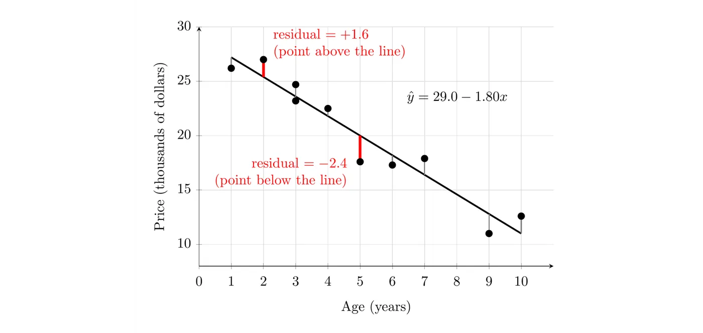
Example 1: Residuals for two used cars

The model for the used cars from Topic 5.1 is

\hat{y} = 29.0 - 1.80x

(

x

= age in years,

\hat{y}

= predicted price in thousands of dollars). Car 6 is 5 years old and listed at 17.6 thousand dollars. Find and interpret its residual.

Step 1: Find the predicted price for

x = 5

\hat{y} = 29.0 - 1.80(5) = 29.0 - 9.0 = 20.0

Step 2: Subtract predicted from actual.

\text{residual} = y - \hat{y} = 17.6 - 20.0 = -2.4

Answer: This car's listed price is $2,400 less than the model predicts for a 5-year-old car.

Car 2 is 2 years old and listed at 27.0 thousand dollars. Its predicted price is

\hat{y} = 29.0 - 1.80(2) = 25.4

, so its residual is

27.0 - 25.4 = 1.6

: it's listed $1,600 more than the model predicts for a 2-year-old car.

What the sign of a residual tells you

Residual	The point is	The model
Positive	above the line (actual > predicted)	underpredicts (underestimates) $y$
Negative	below the line (actual < predicted)	overpredicts (overestimates) $y$
Zero	on the line	predicts $y$ exactly

Template: "The actual [response] was [size of residual, with units] [higher/lower] than the model predicted for [the individual's

x

-value, in context]."

Example 2: Working backward from a residual (AP-style)

Suppose a biologist measured 20 wolves and found the model

\hat{y} = -42.96 + 0.5084x

, where

x

is body length in centimeters and

\hat{y}

is predicted weight in kilograms. One wolf is 160 cm long and has a residual of

-4.6

kg.

(a) What is this wolf's actual weight?

First find the predicted weight:

\hat{y} = -42.96 + 0.5084(160) = -42.96 + 81.344 \approx 38.38

Since residual

= y - \hat{y}

, the actual weight is the predicted weight plus the residual:

y = \hat{y} + \text{residual} = 38.38 + (-4.6) = 33.78

The wolf weighs about 33.78 kg.

(b) Interpret the residual.

This wolf weighs 4.6 kg less than the model predicts for a wolf that is 160 cm long. The model overestimates its weight.

Residual plots

A residual plot is a scatterplot of the residuals versus the predicted response values (

\hat{y}

), or versus the explanatory variable values (

x

). A horizontal line at residual = 0 stands for the regression line. The plot "flattens out" the linear trend so you can see what's left over.

Here are the residuals for all 10 cars:

Age $x$ (years)	Price $y$	Predicted $\hat{y}$	Residual $y - \hat{y}$
1	26.2	27.2	$-1.0$
2	27.0	25.4	$1.6$
3	23.2	23.6	$-0.4$
3	24.7	23.6	$1.1$
4	22.5	21.8	$0.7$
5	17.6	20.0	$-2.4$
6	17.3	18.2	$-0.9$
7	17.9	16.4	$1.5$
9	11.0	12.8	$-1.8$
10	12.6	11.0	$1.6$

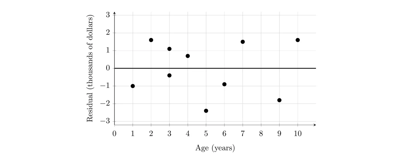
For a simple linear regression, plotting against

x

or against

\hat{y}

shows the same pattern. With a negative slope, the

\hat{y}

version is flipped left to right (older cars have smaller predicted prices), but the shape is the same. Also notice that the residuals add up to 0. For a least-squares line (Topic 5.5) they always do, so the points balance above and below the zero line.

On the TI-84: after you run LinReg(a+bx), the calculator stores the residuals in a list called RESID. In STAT PLOT, keep Xlist as L1 and set Ylist to RESID (press 2nd > STAT (LIST) and choose RESID from NAMES). Then ZOOM > 9:ZoomStat.

Using a residual plot to judge a linear model

Residual plots are how you investigate whether a linear regression model is appropriate for the data. A linear model should only be fit if the data have a linear trend, and the residual plot is the check.

Apparent randomness (no pattern, points scattered above and below 0) confirms the linear form. The simple linear regression model is appropriate. The car residual plot above looks like this: no curve, no trend, just scatter.

Curvature (a U shape, an upside-down U, or a wave) means the linear model is not the most appropriate model. The line runs too low in some places and too high in others, so a curved model would fit better.

Why bother, if you already have a scatterplot? The residual plot magnifies whatever pattern the line misses. A scatterplot can look nearly linear while its residual plot shows a clear curve.

Example 3: Stopping distance (AP-style)

Suppose an engineer measured a car's stopping distance (feet) at 11 speeds from 20 to 70 mph. The least-squares line is

\hat{y} = -93.14 + 5.955x

, where

x

is speed in mph, with

r = 0.99

. The scatterplot and residual plot are below.

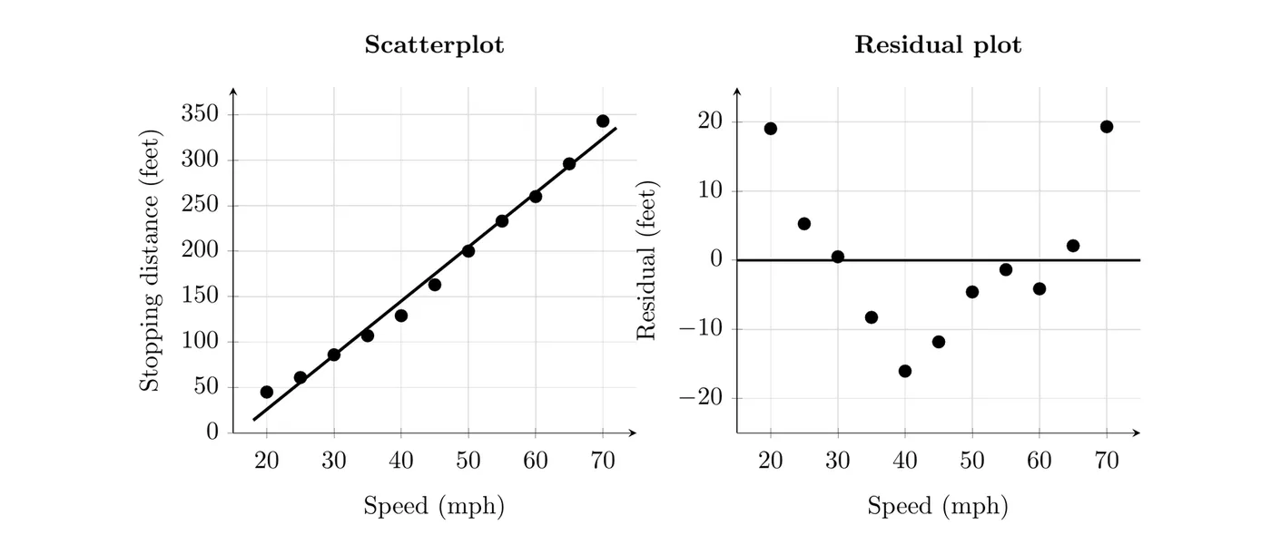
Is a linear model appropriate for these data? Justify your answer.

Answer: No. Even though

r = 0.99

and the scatterplot looks close to linear, the residual plot shows a clear curved (U-shaped) pattern: the residuals are positive at low speeds, negative at middle speeds, and positive again at high speeds. Curvature in the residual plot means a linear model is not the most appropriate model for the relationship between speed and stopping distance. The line underpredicts stopping distance at the lowest and highest speeds and overpredicts it in the middle. (This matches physics: braking distance grows with the square of speed.)

Common mistakes

Computing $\hat{y} - y$ instead of $y - \hat{y}$ . A residual is actual minus predicted.

Mixing up over and under. A negative residual means the model overpredicted.

Trusting a high $r$ without the residual plot. Example 3 has $r = 0.99$ and the wrong model.

Reading a residual plot like a scatterplot of the data. Its vertical axis is prediction error, not the response.

Saying only "random." Describe what you see: "no curved pattern; the residuals are scattered above and below 0."

Interpreting a residual without units or context.

Back Next