5.5 - Least-Squares Regression

Overview

Many lines could be drawn through a scatterplot. The one AP Statistics uses is the least-squares regression line (LSRL), the line that makes the squared prediction errors as small as possible. This topic covers what "least squares" means, how to get the line,

r

, and

r^2

from technology or computer output, and how to interpret the slope, the

y

-intercept, and

r^2

in context. Those interpretations show up on almost every AP exam.

The least-squares idea

The simple linear regression model is fit to the data by minimizing the sum of the squares of the residuals. That's why the result is called the least-squares regression line (LSRL), or the line of best fit.

Why squares? Residuals are positive and negative, so plain residuals would cancel out. (For the LSRL they add to exactly 0.) Squaring makes every miss count as a positive amount, and it makes big misses count much more than small ones.

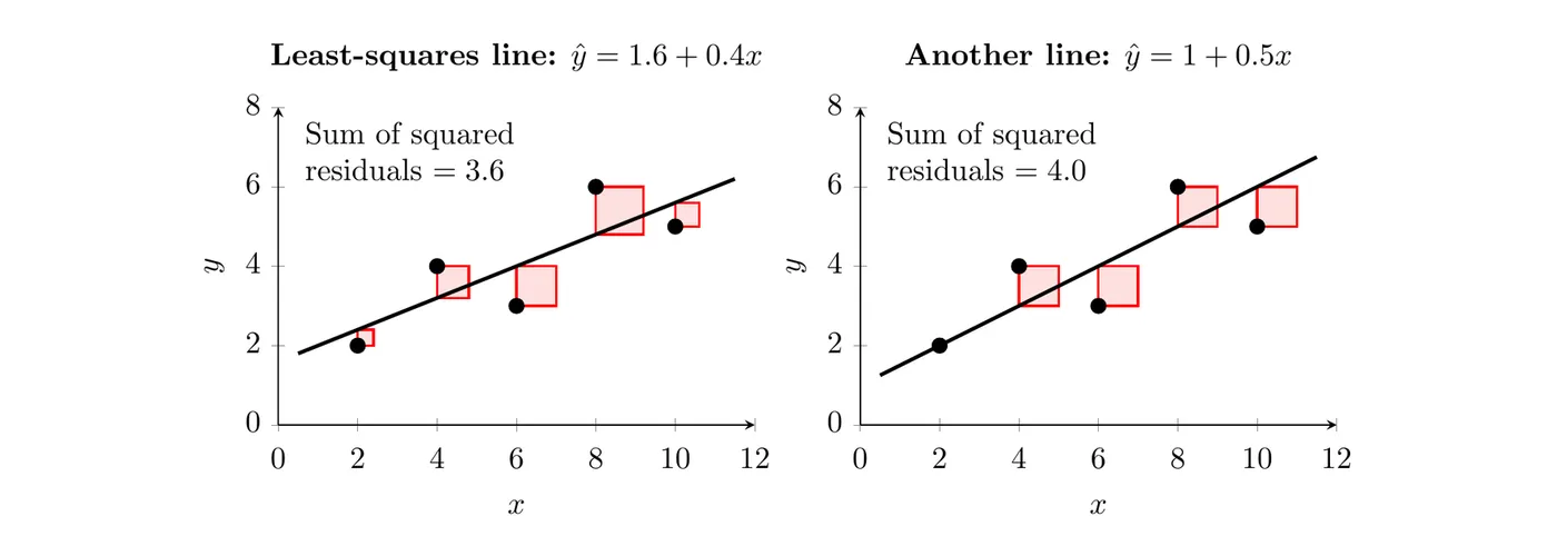
In the figure, each red square has a side as long as one residual, so its area is that residual squared. For the least-squares line on the left, the residuals are

-0.4

0.8

-1.0

1.2

, and

-0.6

(-0.4)^2 + 0.8^2 + (-1.0)^2 + 1.2^2 + (-0.6)^2 = 0.16 + 0.64 + 1.00 + 1.44 + 0.36 = 3.6

The line on the right looks just as reasonable by eye, but its residuals (

0

1

-1

1

-1

) give a total of 4.0. No line through these five points gets the total below 3.6, and that's exactly what makes the left line the least-squares line.

The LSRL passes through the point of means

The least-squares line always passes through the point

(\bar{x}, \bar{y})

. Plug in

x = \bar{x}

, and the model predicts

\hat{y} = \bar{y}

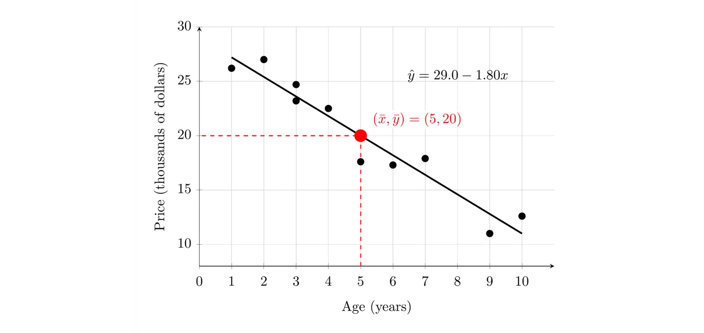
For the used cars from Topic 5.1,

\bar{x} = 5.0

years and

\bar{y} = 20.0

thousand dollars, and

\hat{y} = 29.0 - 1.80(5.0) = 20.0

. This fact is handy when a problem gives you the means and the slope but not the intercept.

Example 1: Finding the intercept from the means

The 10 used cars have mean age 5.0 years and mean price 20.0 thousand dollars, and the slope of the LSRL is

-1.80

. Find the

y

-intercept.

Since

(\bar{x}, \bar{y})

is on the line, substitute it into

\hat{y} = a + bx

20.0 = a + (-1.80)(5.0) \quad\Rightarrow\quad 20.0 = a - 9.0 \quad\Rightarrow\quad a = 29.0

Answer:

a = 29.0

, so the LSRL is

\hat{y} = 29.0 - 1.80x

Getting $a$ , $b$ , $r$ , and $r^2$ from technology

In this course, the slope

b

, the

y

-intercept

a

, and the correlation

r

are all calculated with technology. The formula sheet only gives

\hat{y} = a + bx

. The slope and

r

always have the same sign.

On the TI-84:

Enter the $x$ -values in L1 and the $y$ -values in L2 (STAT > 1:Edit).

Turn on diagnostics once so $r$ and $r^2$ show up: MODE, set STAT DIAGNOSTICS to ON (on older models: 2nd > 0 for CATALOG, choose DiagnosticOn, press ENTER twice).

Press STAT > CALC > 8:LinReg(a+bx). Set Xlist to L1 and Ylist to L2. To graph the line too, set Store RegEQ to Y1 (VARS > Y-VARS > 1:Function > Y1). Choose Calculate.

For the cars, the calculator shows:

TI-84 shows	What it is	Used cars
a	$y$ -intercept	29.0
b	slope	$-1.80$
r²	coefficient of determination	0.928
r	correlation coefficient	$-0.963$

Reading computer output

AP questions often give computer regression output instead of a calculator screen. Here is the output for the 20 wolves from Topic 5.4 (lengths from 142 to 188 cm):

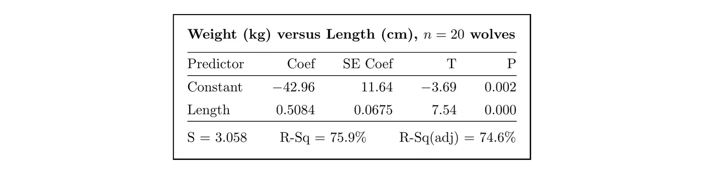
The Coef in the Constant row is the $y$ -intercept: $a = -42.96$ .

The Coef in the row named for the explanatory variable (here, Length) is the slope: $b = 0.5084$ .

R-Sq is $r^2$ : here 75.9%, or 0.759.

So the LSRL is

\hat{y} = -42.96 + 0.5084x

, or predicted weight =

-42.96 + 0.5084

(length). The other entries (SE Coef, T, P, and R-Sq(adj)) are for inference and model comparisons beyond this course, so you can skip them. S is the typical size of a residual, about 3.06 kg here. The most common slip is reading the slope from the Constant row: the slope is always in the row with the variable's name.

The output doesn't show

r

, but you can get it from

r^2

: take the square root and give it the same sign as the slope. Here,

r = +\sqrt{0.759} \approx 0.871

, positive because the slope is positive.

Interpreting the slope

The slope

b

is the predicted increase or decrease in the response variable for a one-unit increase in the explanatory variable. Always interpret it in context.

Template: "For each additional [1 unit of

x

], the predicted [response] increases (or decreases) by [

|b|

and units]."

Cars (

b = -1.80

): For each additional year of age, the predicted price of the car decreases by 1.80 thousand dollars ($1,800).

Two words do a lot of work here. "Predicted" (or "on average") shows that the slope describes the model's trend, not a guarantee for every individual. "For each additional" shows it's a rate: change per one unit of

x

, not just "a change." Leaving either one out costs credit.

Interpreting the $y$ -intercept

The

y

-intercept

a

is the predicted value of the response variable when the explanatory variable is 0, interpreted in context.

Template: "When [

x

in context] is 0, the predicted [response] is [

a

and units]."

Sometimes the intercept has no reasonable meaning, for two reasons:

$x = 0$ is outside the interval of $x$ -values used to find the line, so interpreting $a$ is an extrapolation.

The predicted value is impossible, like a negative weight or height.

Cars (

a = 29.0

): A car that is 0 years old (new) has a predicted price of 29.0 thousand dollars ($29,000). Age 0 is just below the data's range (1 to 10 years), so this is a small extrapolation: reasonable, but treat it with some caution.

For the wolves, the intercept is a predicted weight of

-42.96

kg, which has no meaning (Example 2 explains why). AP questions often say "interpret the intercept, or explain why it isn't meaningful." Either way, you need context.

The coefficient of determination, $r^2$

In simple linear regression, the square of the correlation coefficient,

r^2

, is called the coefficient of determination. It's the proportion of the variation in the response variable that is explained by the linear relationship with the explanatory variable.

Template: "About [

r^2

as a percent] of the variation in [response] is explained by the linear relationship with [explanatory variable]."

Cars (

r^2 = 0.928

): About 92.8% of the variation in the listed prices of these cars is explained by the linear relationship with age. The other 7.2% comes from things the model leaves out, like mileage and condition.

Where $r^2$ comes from

Without the model, your best guess for every car's price is

\bar{y} = 20.0

, and the squared distances from

\bar{y}

add up to 279.24 (the total variation in price). Using age, the squared residuals add up to only 20.04, so the line accounts for

r^2 = 1 - \frac{20.04}{279.24} \approx 0.928

Some things to remember about

r^2

$0 \le r^2 \le 1$ . It's never negative, so it can't show direction. Get the direction from the sign of the slope.

It's about variation in the response ( $y$ ), not in $x$ . Multiple-choice questions love to swap the two.

A high $r^2$ doesn't prove a linear model is appropriate. That's the residual plot's job (Topic 5.4).

The coefficients are statistics

The slope

b

and the

y

-intercept

a

of the least-squares line are statistics, because they're calculated from a sample of data, not from the whole population. A different sample gives a different line: another 10 used cars of the same model would give a slightly different slope and intercept. The LSRL from a sample estimates the true relationship in the population, the same way

\bar{x}

estimates

\mu

Putting it together

Example 2: Wolves (AP-style)

Use the computer output for the 20 wolves above (body lengths from 142 to 188 cm).

(a) Write the equation of the least-squares regression line. Define any variables you use.

\hat{y} = -42.96 + 0.5084x

, where

x

is body length in centimeters and

\hat{y}

is predicted weight in kilograms.

(b) Interpret the slope in context.

For each additional centimeter of body length, the predicted weight of a wolf increases by about 0.508 kg.

(c) Interpret the

y

-intercept, or explain why it isn't meaningful.

It would be the predicted weight of a wolf with a body length of 0 cm,

-42.96

kg. That isn't meaningful. No wolf has length 0, a length of 0 is far outside the data (142 to 188 cm), so it's an extrapolation, and a weight can't be negative. Here the intercept only places the line.

(d) Interpret

r^2

, and find the correlation.

About 75.9% of the variation in wolf weight is explained by the linear relationship with body length. Since the slope is positive,

r = +\sqrt{0.759} \approx 0.871

: a strong, positive linear association between body length and weight.

(e) Predict the weight of a wolf that is 175 cm long.

\hat{y} = -42.96 + 0.5084(175) = -42.96 + 88.97 = 46.01

The model predicts about 46.0 kg. Since 175 cm is inside the range of lengths in the data (142 to 188 cm), this is an interpolation.

Example 3: Finding $r$ from $r^2$ and the slope

A least-squares line has slope

b = -0.6

and

r^2 = 0.49

. What is

r

Answer:

\sqrt{0.49} = 0.7

, and

r

has the same sign as the slope, which is negative. So

r = -0.7

, a moderate negative linear association.

Common mistakes

Interpreting the slope without "predicted" (or "on average"), or without "for each additional unit."

Reading the slope from the Constant row. The slope is in the row named for the explanatory variable.

Taking the positive square root of $r^2$ when the slope is negative. $r$ always has the slope's sign.

Calling $r^2$ the variation in $x$ , or "the percent of points on the line." It's the proportion of variation in $y$ explained by the linear relationship with $x$ .

Interpreting an intercept that's impossible or an extrapolation without saying so.

Forgetting that the LSRL passes through $(\bar{x}, \bar{y})$ , which can give you a missing intercept.

BackNext

5.5 - Least-Squares Regression

Overview

The least-squares idea

The LSRL passes through the point of means

Example 1: Finding the intercept from the means

Getting aaa, bbb, rrr, and r2r^2r2 from technology

Reading computer output

Interpreting the slope

Interpreting the yyy-intercept

The coefficient of determination, r2r^2r2

Where r2r^2r2 comes from

The coefficients are statistics

Putting it together

Example 2: Wolves (AP-style)

Example 3: Finding rrr from r2r^2r2 and the slope

Common mistakes

Getting $a$ , $b$ , $r$ , and $r^2$ from technology

Interpreting the $y$ -intercept

The coefficient of determination, $r^2$

Where $r^2$ comes from

Example 3: Finding $r$ from $r^2$ and the slope