1.3 - Representing Motion

Ways to Represent Motion

Motion can be described in a bunch of different ways:

Equations: the math relationships between variables

Graphs: visual plots of position, velocity, or acceleration over time

Motion diagrams: dots showing position at equal time intervals

Figures: pictures or diagrams of the situation

Narrative descriptions: just explaining it in words

This section focuses on equations and graphs, since the two are closely connected.

Motion Diagrams

Motion diagrams use dots to mark an object’s position at equally spaced time intervals, like every 0.5 seconds.

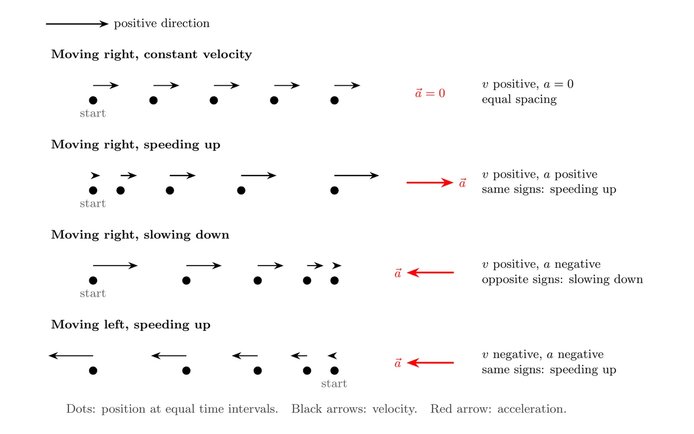
Here’s how to read the spacing:

equal spacing means constant velocity, no acceleration

increasing spacing means speeding up (acceleration points the same way the object is moving)

decreasing spacing means slowing down (acceleration points opposite to the motion)

The spacing between dots is basically the displacement during that time interval, and since the time intervals themselves stay the same, bigger gaps mean higher velocity.

Speeding up or slowing down? The sign of acceleration alone can’t tell you. Compare the signs of velocity and acceleration (the black and red arrows in the motion diagrams above):

Same signs (both $+$ or both $-$ ): speeding up

Opposite signs: slowing down

So “negative acceleration” doesn’t automatically mean slowing down. A car moving in the negative direction that speeds up has a negative velocity and a negative acceleration.

Constant Acceleration Kinematic Equations (CAKE)

Most intro physics problems assume constant acceleration, which lets us use three powerful equations to solve almost anything.

There are five kinematic variables in play: final velocity

v

, initial velocity

v_0

, acceleration

a

, displacement

\Delta x

, and time

t

. Each of the three equations below uses four of these five variables, leaving one out.

Equation 1 (velocity as a function of time), missing $\Delta x$ :

v = v_0 + at

Use this when you need velocity and don’t know displacement.

Equation 2 (position as a function of time), missing $v$ :

\Delta x = v_0 t + \frac{1}{2}at^2

Or written the way formula sheets show it:

x = x_0 + v_0 t + \frac{1}{2}at^2

Use this when you need displacement and don’t know the final velocity. It’s a quadratic in time.

Equation 3, the “timeless” equation, missing $t$ :

v^2 = v_0^2 + 2a\Delta x

Use this when you need to connect velocity and displacement without touching time at all.

Picking the right one: figure out which variable you don’t have and don’t need, then grab the equation that leaves that variable out. If you don’t know the final velocity and don’t need it, use Equation 2. If you don’t know the time and don’t need it, use Equation 3. If you don’t know the displacement and don’t need it, use Equation 1.

How they look on the AP equation sheet:

v_x = v_{x0} + a_x t

x = x_0 + v_{x0} t + \frac{1}{2} a_x t^2

, and

v_x^2 = v_{x0}^2 + 2a_x (x - x_0)

These are the same three equations (

x - x_0

is just

\Delta x

). The

x

subscript is only a label, so for up-and-down motion use the same equations with

y

. They only work while acceleration stays constant. If the motion has stages (speeding up, then cruising, then braking), apply them one stage at a time, using the final velocity of one stage as the initial velocity of the next.

Free Fall and Gravity

Near Earth’s surface, everything accelerates downward at the same constant rate, no matter its mass.

g = 9.8 \text{ m/s}^2 \approx 10 \text{ m/s}^2

This acceleration is constant in magnitude, always points down, and is the same for every object (ignoring air resistance).

If you set up your coordinate system with up as positive, then:

a = -g = -10 \text{ m/s}^2

The negative sign is just marking the downward direction.

Whenever a problem needs a number for

g

, the AP Physics 1 course framework says “the value

g = 10 \text{ m/s}^2

will be used,” and you won’t be penalized for using the more precise

9.8 \text{ m/s}^2

9.81 \text{ m/s}^2

instead. (The equation sheet itself prints

g = 9.8 \text{ m/s}^2

.) Pick one value and stay consistent within a problem. Anything falling, thrown, or launched (with air resistance ignored) has this acceleration.

Worked Example: Dropping an Object

A drone drops a sensor package from rest. It falls freely for 4 seconds before the parachute opens. Using

g = 10 \text{ m/s}^2

, find how far it fell and how fast it’s going right before the parachute deploys.

Finding displacement:

We know

v_0 = 0

(dropped from rest),

t = 4

a = -10 \text{ m/s}^2

, and

x_0 = 0

at the release point.

Since we want displacement and don’t know the final velocity, use Equation 2:

\Delta x = v_0 t + \frac{1}{2}at^2

Since

v_0 = 0

, that whole first term drops out (a common mistake is forgetting to drop the entire

v_0 t

term, not just the

v_0

\Delta x = \frac{1}{2}at^2 = \frac{1}{2}(-10)(4)^2 = \frac{1}{2}(-10)(16) = -80 \text{ m}

So the package falls 80 meters, and the negative sign just tells us it’s below where it started.

Finding final velocity:

We want final velocity and we have time, so use Equation 1:

v = v_0 + at

Since

v_0 = 0

v = at = (-10)(4) = -40 \text{ m/s}

So the package is moving at 40 m/s downward right before the parachute opens.

Double checking with Equation 3:

Even though Equation 3 also works here, it’s smarter to verify using earlier results rather than relying on them, since an error in Part 1 would carry over into Part 2 if you use

\Delta x

to find velocity.

v^2 = 0^2 + 2(-10)(-80) = 1600 \implies v = -40 \text{ m/s} \checkmark

(We pick the negative root since we know the motion is downward.)

Worked Example: Braking Distance

A car moving at 24 m/s brakes to a stop with a constant acceleration of magnitude

6.0 \text{ m/s}^2

. How far does it travel while braking?

Setup: the direction of motion is positive, so

v_0 = +24

m/s,

v = 0

(it stops), and

a = -6.0 \text{ m/s}^2

(slowing down, so opposite the motion). We want

\Delta x

and don’t know

t

, so use Equation 3:

v^2 = v_0^2 + 2a\Delta x \implies 0 = (24)^2 + 2(-6.0)\Delta x

\Delta x = \frac{-(24)^2}{2(-6.0)} = \frac{-576}{-12} = 48 \text{ m}

What if the car were going twice as fast? Solving Equation 3 for distance gives

\Delta x = \frac{v_0^2}{2|a|}

, so doubling

v_0

makes the braking distance 4 times longer (192 m), not twice as long.

Solving Problems Step by Step

List what you know: write down given values with proper symbols and units

Identify your target: what are you actually solving for

Pick the right equation: the one with your target variable and three known values

Write the equation first: before plugging in numbers, this shows your reasoning and often earns points

Substitute and simplify: cross out zero terms explicitly to avoid mistakes

Calculate and state your answer: include units and direction

Sanity check: does the size and sign of your answer make physical sense

Handy Conventions

For free fall problems, it’s usually easiest to set

x_0 = 0

right at the release point, which eliminates one variable immediately.

“From rest” or “dropped” both mean

v_0 = 0

, which simplifies things a lot:

Equation 1 becomes $v = at$

Equation 2 becomes $\Delta x = \frac{1}{2}at^2$

Equation 3 becomes $v^2 = 2a\Delta x$

And watch the wording: “dropped” means

v_0 = 0

, “thrown downward” means

v_0 < 0

, and “thrown upward” means

v_0 > 0

Worked Example: Thrown Straight Up

A ball is thrown straight up at 15 m/s. Using

g = 10 \text{ m/s}^2

and up as positive, find how long it takes to reach the top, how high it goes, and its velocity when it comes back to the thrower’s hand.

Time to the top: at the highest point the velocity is zero for an instant.

v = v_0 + at \implies 0 = 15 + (-10)t \implies t = 1.5 \text{ s}

Maximum height:

v^2 = v_0^2 + 2a\Delta y \implies 0 = (15)^2 + 2(-10)\Delta y \implies \Delta y = \frac{225}{20} = 11.25 \text{ m} \approx 11 \text{ m}

Back at the hand: the ball returns to where it started, so

\Delta y = 0

0 = 15t + \frac{1}{2}(-10)t^2 = 5t(3 - t) \implies t = 3.0 \text{ s}

v = v_0 + at = 15 + (-10)(3.0) = -15 \text{ m/s}

Same speed as the throw, now pointing down, and the trip down takes as long as the trip up.

Watch out: at the top the velocity is zero, but the acceleration is not. It’s still

-10 \text{ m/s}^2

the whole time. If the acceleration were zero at the top, the ball would just hang there.

Representing Motion: Graphs

Three Main Graph Types

Kinematics relies on three key graphs:

Position vs. time ( $x$ vs. $t$ )

Velocity vs. time ( $v$ vs. $t$ )

Acceleration vs. time ( $a$ vs. $t$ )

Time always goes on the horizontal axis as the independent variable, while position, velocity, or acceleration goes on the vertical axis as the dependent variable, since these quantities change as time moves forward.

Position vs. Time Graphs

These show where an object is at every moment, and they’re basically the graph version of a motion diagram.

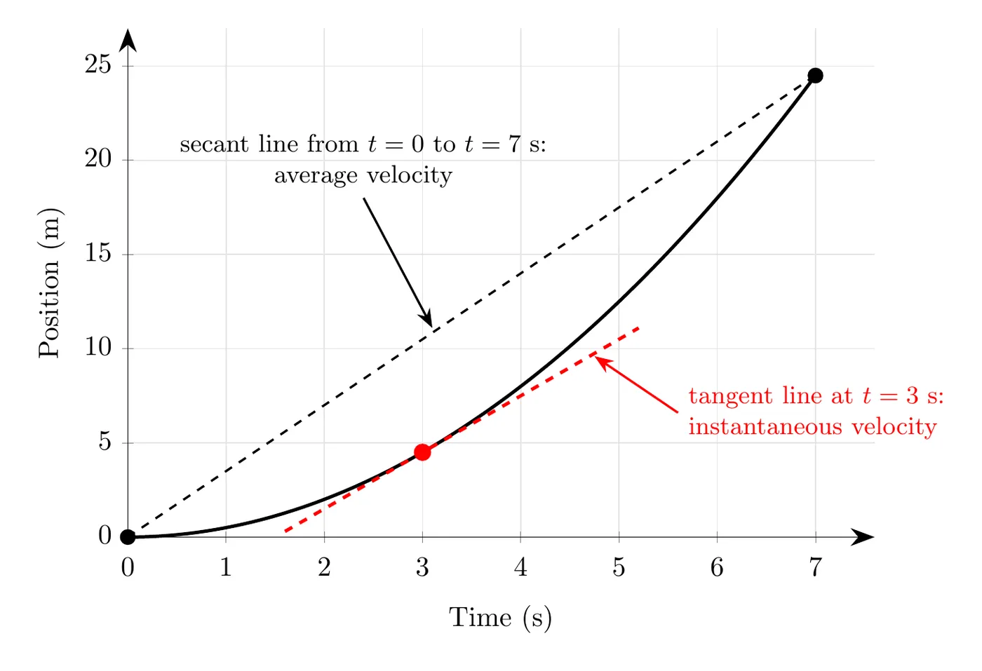
Slope equals velocity:

\text{slope of } x\text{-}t \text{ graph} = \frac{\Delta x}{\Delta t} = v

For instantaneous velocity at a specific point, draw a tangent line at that point, its slope is the instantaneous velocity. For average velocity over an interval, draw a secant line connecting the start and end points, its slope is the average velocity. (Easy way to remember it: “secant connects” two points.)

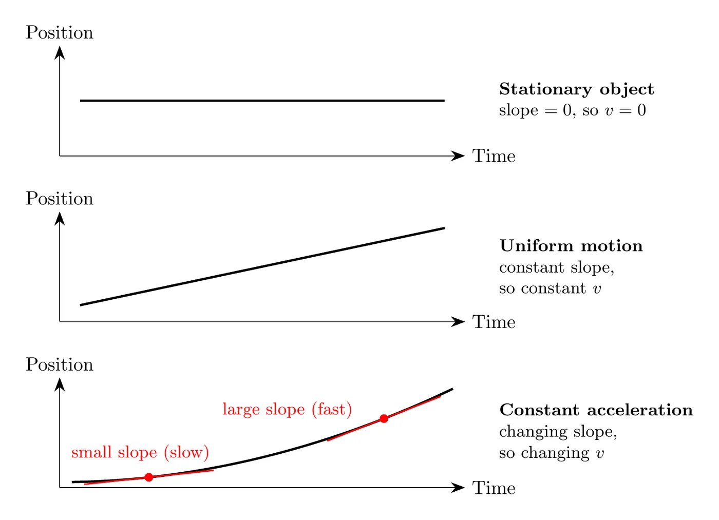
Three cases:

Stationary: horizontal line, slope of 0, velocity is 0, position never changes

Uniform motion: straight line, constant slope, constant velocity, instantaneous velocity equals average velocity everywhere

Accelerated motion: curved line, changing slope, changing velocity, a parabolic shape means constant acceleration

Velocity vs. Time Graphs

This is really the central graph in kinematics since it connects position and acceleration.

Slope equals acceleration:

\text{slope of } v\text{-}t \text{ graph} = \frac{\Delta v}{\Delta t} = a

Tangent line slope gives instantaneous acceleration, secant line slope gives average acceleration.

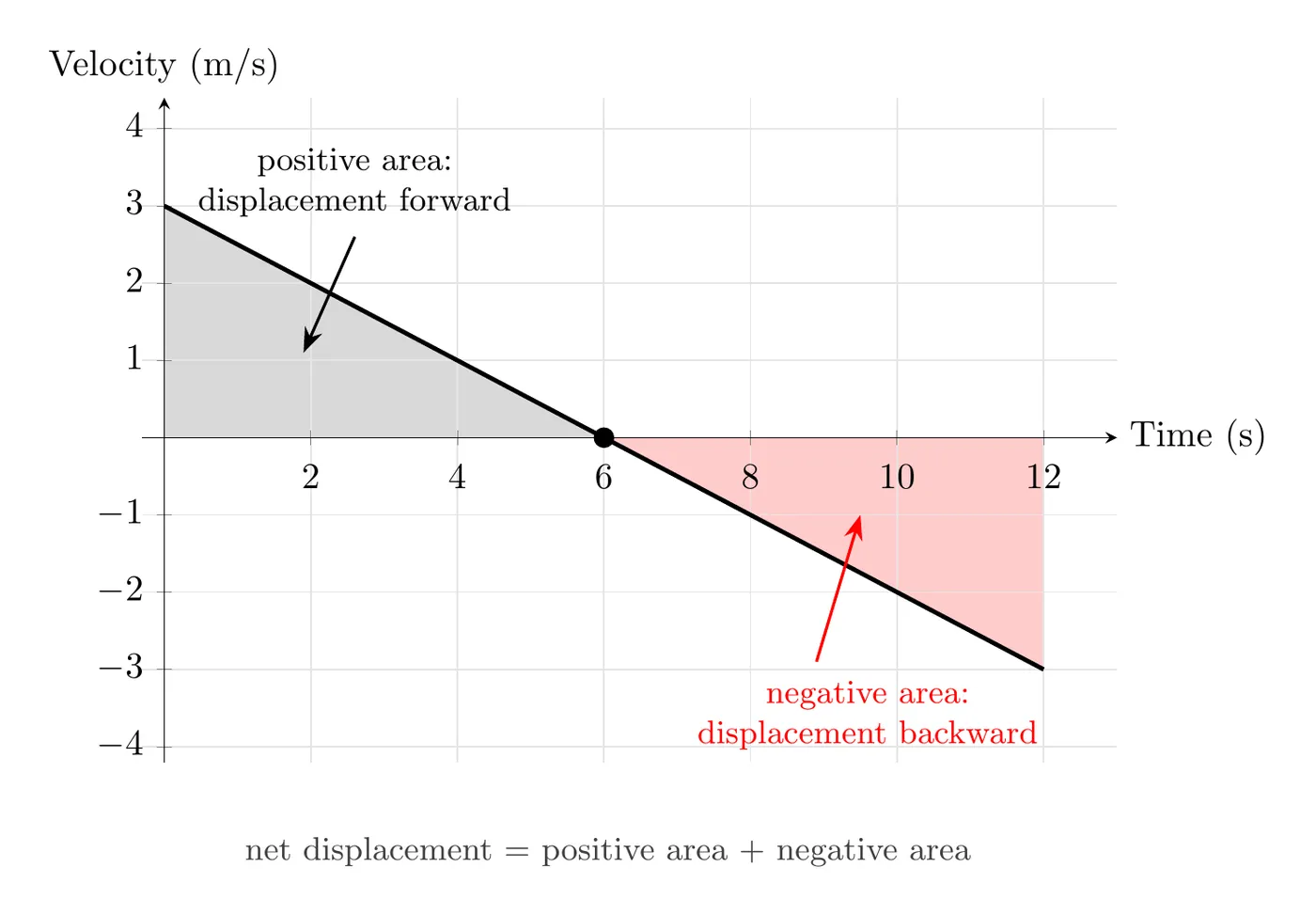
Area under the curve equals displacement:

\text{Area under } v\text{-}t \text{ graph} = \Delta x

This is basically integration happening without formally calling it that: you’re summing up all the tiny displacements (

v \cdot dt

) over time.

Since velocity vs. time graphs in constant acceleration problems are always straight lines, the areas form simple shapes:

Rectangle: area $= \text{base} \times \text{height} = t \times v$

Triangle: area $= \frac{1}{2} \times t \times v$

Trapezoid: split into a rectangle plus a triangle, or use $\frac{1}{2}(b_1 + b_2) \times h$

Watch your scale: a shape that looks square on the graph might actually be a rectangle because the axes use different scales. Always calculate area from the actual axis values, one unit on the time axis might be 1 second while one unit on the velocity axis might be 10 m/s, not from how the shape looks.

Sign of the area:

area above the time axis is positive displacement

area below the time axis is negative displacement

net displacement is the algebraic sum of both

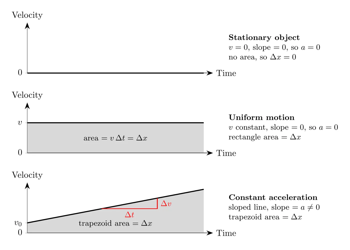
Three cases:

Stationary: horizontal line at $v = 0$ , slope 0 so $a = 0$ , no area so $\Delta x = 0$

Uniform motion: horizontal line at some nonzero $v$ , slope 0 so $a = 0$ , rectangular area gives displacement

Constant acceleration: sloped line, nonzero slope so $a \neq 0$ , triangular or trapezoidal area gives displacement

Acceleration vs. Time Graphs

These are the simplest graphs in constant acceleration kinematics.

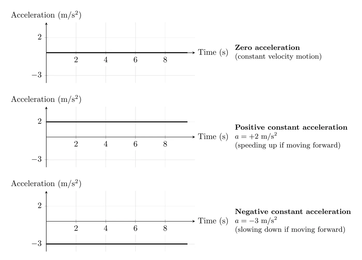
Area under the curve equals change in velocity:

\text{Area under } a\text{-}t \text{ graph} = \Delta v

When acceleration is constant, the acceleration vs. time graph is a horizontal line, whether that value is zero or not. Motion often happens in stages (speed up, cruise, brake), so the graph can be a set of flat steps, one for each stage. A sloped or curved acceleration graph means the acceleration itself is changing. AP Physics 1 won’t ask you to calculate with changing acceleration, but you may need to sketch or explain it (see Nonuniform Acceleration below).

Connecting Graphs and Equations

The kinematic equations are really just the algebra version of the graphs:

Equation	Matching Graph
$v = v_0 + at$	Velocity vs. time (a line)
$\Delta x = v_0 t + \frac{1}{2}at^2$	Position vs. time (a parabola)
$a = \text{constant}$	Acceleration vs. time (horizontal line)

Going between quantities:

Acceleration to velocity: area under $a$ - $t$ graph, or $\Delta v = a \cdot t$

Velocity to position: area under $v$ - $t$ graph, or $\Delta x = v \cdot t$ when velocity is constant

Position to velocity: slope of $x$ - $t$ graph, or $v = \frac{\Delta x}{\Delta t}$

Velocity to acceleration: slope of $v$ - $t$ graph, or $a = \frac{\Delta v}{\Delta t}$

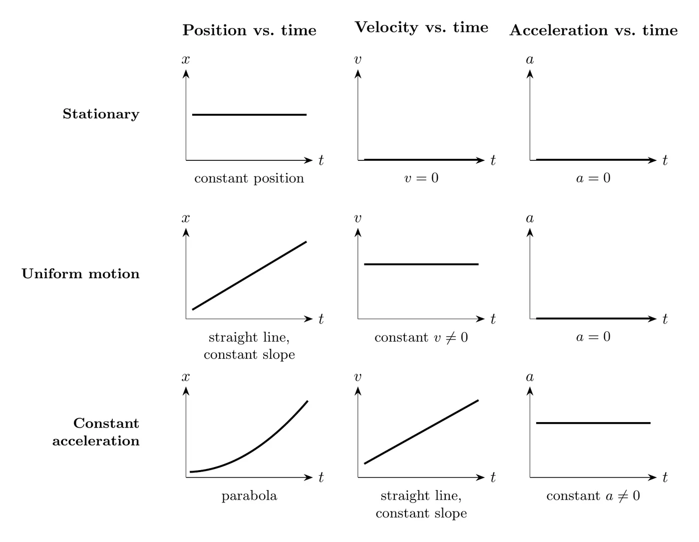
All Three Motion Types Compared

Worked Example: Analyzing a Velocity-Time Graph

A robot’s velocity is tracked for 20 seconds. The graph shows velocity starting at 12 m/s at

t = 0

, decreasing in a straight line to 0 m/s at

t = 10

s, continuing to decrease in a straight line to

-4

m/s at

t = 15

s, then staying flat at

-4

m/s from

t = 15

s to

t = 20

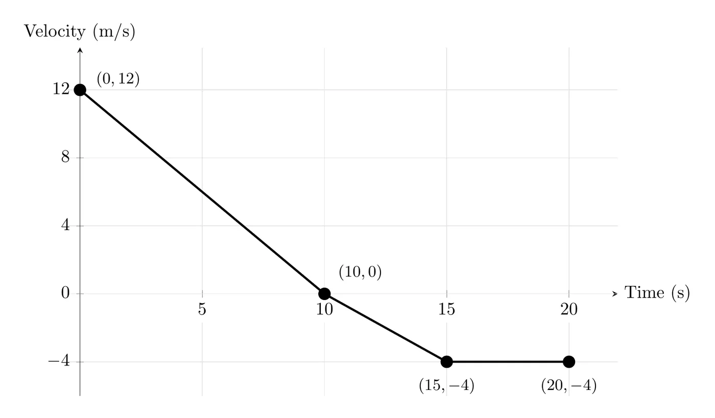
Find the instantaneous acceleration at

t = 7

s, the average acceleration over the first 15 seconds, and the displacement during the first 12 seconds.

Instantaneous acceleration at t = 7 s:

Since the graph is linear from

t = 0

t = 10

s, the slope (acceleration) is constant across that whole stretch. Using the endpoints

(0, 12)

and

(10, 0)

a = \frac{v_f - v_i}{t_f - t_i} = \frac{0 - 12}{10 - 0} = -1.2 \text{ m/s}^2

So at

t = 7

s, the robot is slowing down at

1.2 \text{ m/s}^2

Average acceleration over the first 15 seconds:

Draw a secant from

t = 0

t = 15

s, using the points

(0, 12)

and

(15, -4)

a_{avg} = \frac{-4 - 12}{15 - 0} = \frac{-16}{15} \approx -1.07 \text{ m/s}^2

Displacement during the first 12 seconds:

The tricky part here is that velocity crosses zero at

t = 10

s, which splits things into two regions: a positive triangle from 0 to 10 s, and a negative triangle from 10 to 12 s. A common mistake is only calculating the big triangle out to 15 s instead of stopping at 12 s and accounting for the sign change.

Region 1 (0 to 10 s): base 10 s, height 12 m/s

A_1 = \frac{1}{2}(10)(12) = 60 \text{ m}

Region 2 (10 to 12 s): first find velocity at

t = 12

s, using the slope of the second straight section,

\frac{-4 - 0}{15 - 10} = -0.8 \text{ m/s}^2

, starting from

t = 10

v(12) = 0 + (-0.8)(2) = -1.6 \text{ m/s}

Base 2 s, height

-1.6

m/s:

A_2 = \frac{1}{2}(2)(-1.6) = -1.6 \text{ m}

Net displacement:

\Delta x_{total} = 60 + (-1.6) = 58.4 \text{ m}

So over the first 12 seconds, the robot ends up 58.4 m in the positive direction. It moved forward 60 m during the first 10 seconds, then backward 1.6 m over the next 2 seconds.

Lessons from this example:

When velocity crosses the time axis, motion changes direction, so split your area calculations at those crossing points

Keep the signs, areas below the axis are negative and shouldn’t be treated as positive until you’re combining everything into a net answer

On any straight-line section, instantaneous and average acceleration are the same

Sometimes you need acceleration first just to figure out velocity at some intermediate time

Worked Example: Reading a Position-Time Graph

A cart rolls along a track and slows down steadily until it stops. The graph shows its position, with a tangent line drawn at

t = 2

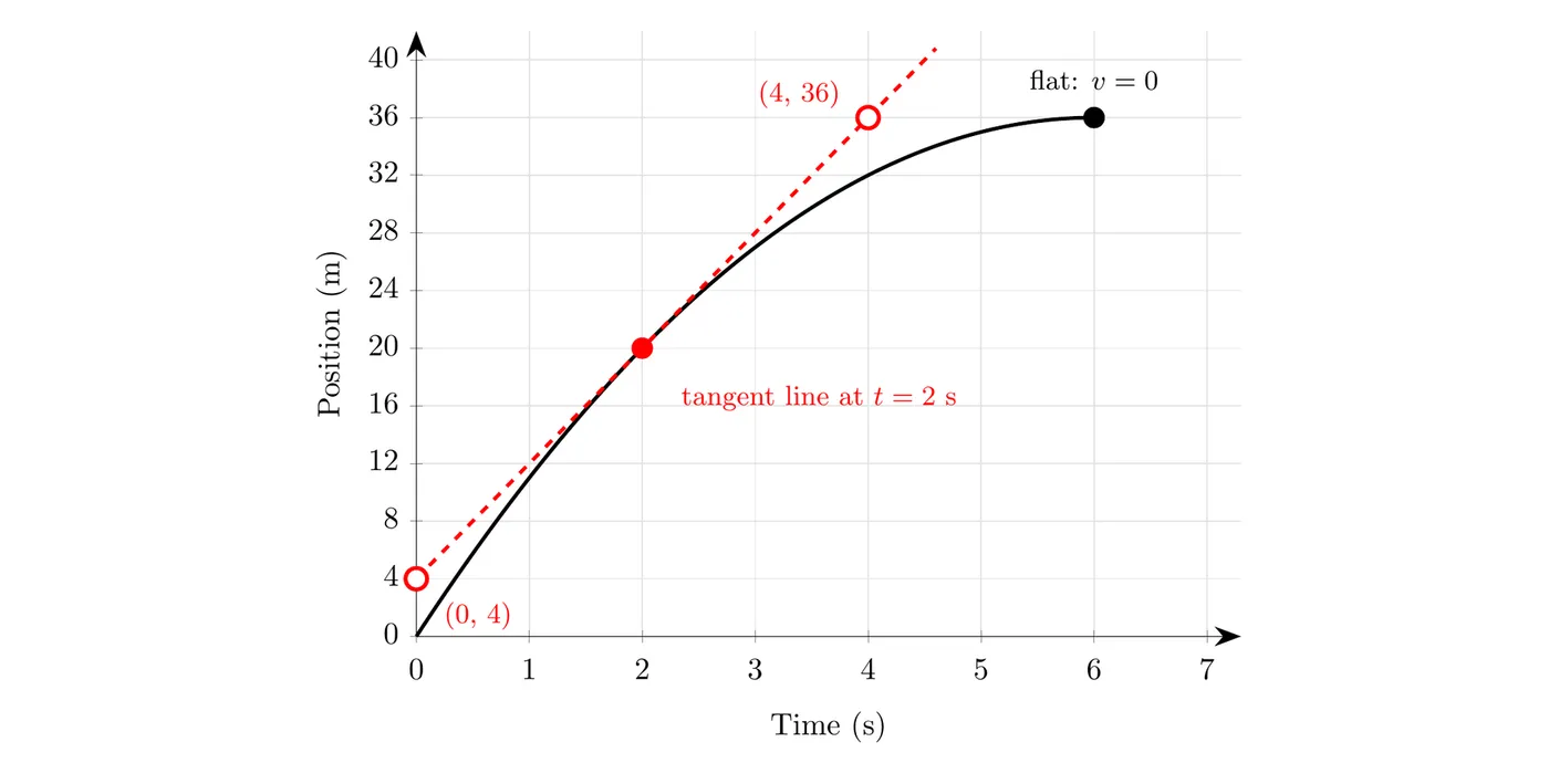
Instantaneous velocity at t = 2 s: pick two points on the tangent line that are far apart and easy to read,

(0, 4)

and

(4, 36)

v = \text{slope of tangent} = \frac{36 - 4}{4 - 0} = \frac{32 \text{ m}}{4 \text{ s}} = 8.0 \text{ m/s}

Average velocity from 0 to 6 s: use the secant line between the curve’s endpoints,

(0, 0)

and

(6, 36)

v_{avg} = \frac{36 - 0}{6 - 0} = 6.0 \text{ m/s}

When is the cart at rest? Where the tangent line is horizontal (slope zero): at

t = 6

s, the top of the curve.

Average acceleration from 2 s to 6 s: the velocity drops from 8.0 m/s to 0, so

a_{avg} = \frac{0 - 8.0}{6 - 2} = -2.0 \text{ m/s}^2

. The negative sign matches the graph: its slope keeps getting smaller.

Notice the instantaneous velocity at 2 s (8.0 m/s) is bigger than the average over the whole trip (6.0 m/s). That makes sense: the cart is slowing down, so it moves fastest early on.

Worked Example: Reading an Acceleration-Time Graph

A subway train starts from rest. It speeds up at

+1.2 \text{ m/s}^2

for 10 s, cruises for 20 s, then brakes at

-1.5 \text{ m/s}^2

for 8.0 s. Find its velocity at the end of each stage, its velocity at

t = 34

s, and how far it travels.

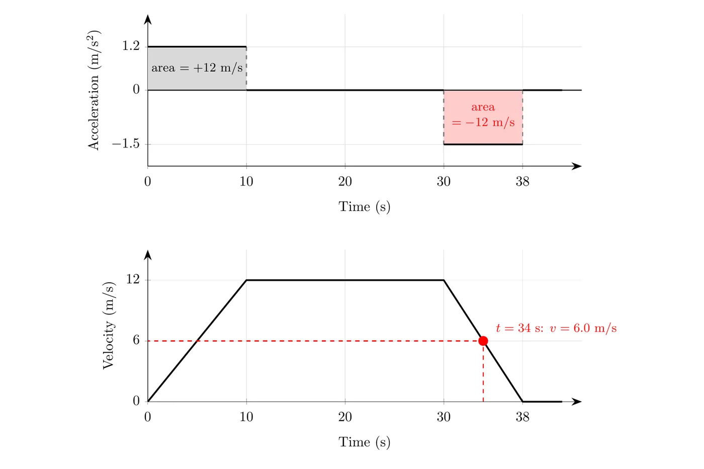
Area under the $a$ - $t$ graph is the change in velocity. Each stage is a rectangle:

0 to 10 s: $\Delta v = (1.2)(10) = +12$ m/s, so $v = 0 + 12 = 12$ m/s

10 to 30 s: $a = 0$ , so there’s no area and $v$ stays at 12 m/s

30 to 38 s: $\Delta v = (-1.5)(8.0) = -12$ m/s, so $v = 12 - 12 = 0$ (the train stops)

Velocity at t = 34 s: that’s 4.0 s into braking, so

\Delta v = (-1.5)(4.0) = -6.0

m/s and

v = 12 - 6.0 = 6.0

m/s. You can read the same value off the velocity graph.

Distance traveled: now use the area under the

v

t

graph (a triangle, a rectangle, and a triangle):

\Delta x = \frac{1}{2}(10)(12) + (20)(12) + \frac{1}{2}(8.0)(12) = 60 + 240 + 48 = 348 \text{ m} \approx 3.5 \times 10^2 \text{ m}

That’s the full chain: the area under the

a

t

graph gives the change in velocity, and the area under the

v

t

graph gives the displacement.

Nonuniform Acceleration (Qualitative Only)

AP Physics 1 won’t ask you to calculate motion with changing acceleration (the kinematic equations don’t apply), but you do need to sketch graphs for it and explain what’s happening. The graph rules stay the same: the slope of

x

t

is velocity, the slope of

v

t

is acceleration, and the area under

v

t

is displacement.

Example: a car pulls away from a stoplight. The driver presses hard on the gas at first, then eases off as the car gets close to the speed limit, so the acceleration shrinks over time.

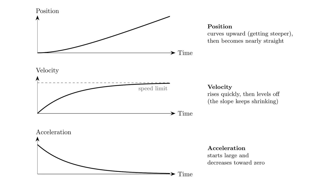
Velocity vs. time: rises steeply at first, then levels off at the speed limit. It’s a curve, not a straight line, because its slope (the acceleration) keeps decreasing.

Acceleration vs. time: starts large and decreases toward zero.

Position vs. time: curves upward as the car gets faster, then becomes nearly a straight line once the velocity stops changing.

Quick test: a straight

v

t

line, no matter how steep, means constant acceleration. A curved

v

t

graph means the acceleration is changing.

Common Graph Mistakes

Mixing up slope and height: thinking a taller point on a velocity graph means bigger acceleration. Acceleration is the slope of that graph, not its height. A high but constant velocity actually has zero acceleration.

Ignoring negative areas: adding every area as if it were positive. Areas below the time axis are negative and represent motion in the opposite direction, so they need to be added algebraically, not just summed as absolute values.

Estimating area visually: assuming a shape is a square just because it looks like one, then using

s^2

. Always pull the real numbers off the axes. A shape that looks 4 by 4 on the page might actually represent 4 seconds by 40 m/s, which is 160 m.

Assuming any two points give instantaneous velocity: connecting two points on a curved position-time graph only gives you the average velocity over that stretch. Instantaneous velocity needs a tangent line at one single point.

Key Takeaways

Equations:

There are five ways to represent motion: equations, graphs, motion diagrams, figures, and narrative descriptions

In motion diagrams, equal spacing means constant velocity, increasing spacing means speeding up, decreasing spacing means slowing down

Same signs for velocity and acceleration means speeding up; opposite signs means slowing down

The three CAKE equations each leave out one of five variables: $v = v_0 + at$ (no $\Delta x$ ), $\Delta x = v_0 t + \frac{1}{2}at^2$ (no $v$ , quadratic in $t$ ), $v^2 = v_0^2 + 2a\Delta x$ (no $t$ )

Gravitational acceleration is $g = 9.8 \text{ m/s}^2 \approx 10 \text{ m/s}^2$ , constant and downward

Use $a = -g$ when up is your positive direction

Free fall just means gravity is the only thing acting, so acceleration is $\pm g$

“From rest” means $v_0 = 0$ , which simplifies everything

Always write the equation before plugging in numbers, and cross out zero terms explicitly

Pick equations based on which values you already know, to avoid carrying errors forward

Graphs:

Time is always the independent variable (x-axis) in kinematics graphs

On position vs. time graphs, slope gives velocity (tangent for instantaneous, secant for average)

On velocity vs. time graphs, slope gives acceleration and area gives displacement

On acceleration vs. time graphs, area gives the change in velocity

Stationary, uniform, and accelerated motion each have distinct signatures across all three graph types

Tangent lines give instantaneous rates, secant lines give average rates

Area above the time axis is positive displacement, area below is negative

Always use actual axis values for area calculations, not visual appearance

Split area calculations wherever a curve crosses the time axis

Equations and graphs are just two different ways of showing the same physics

Under constant acceleration, position graphs are parabolas, velocity graphs are straight lines, and acceleration graphs are horizontal lines

Nonuniform acceleration: sketch and explain it with the same slope and area rules, but don’t use the kinematic equations

Back Next