1.3 - Electric Fields

Where Electric Fields Come From

Electric fields originate from all charged particles. Every charged object creates an electric field in the space around it, the same way a massive object creates a gravitational field.

The key distinction from gravity: - Gravitational fields always pull toward the massive object, so they’re attractive only. - Electric fields can push away from or pull toward the charged object, depending on the sign of the charge.

The Mathematical Definition

The electric field at a point in space is the ratio of the electric force a test charge feels there to the charge of that test charge:

\vec{E} = \frac{\vec{F}_e}{q}

where: -

\vec{E}

= electric field (N/C) -

\vec{F}_e

= electric force on the test charge (N) -

q

= charge of the test charge, sign included (C)

Units: newtons per coulomb (N/C).

A test charge is a point charge small enough that it doesn’t noticeably push around the charges that create the field. If it did, it would change the very field you’re trying to measure. The field at a point is set by the source charges, and it’s there whether or not you put a test charge in it.

The Alternative Form

Rearranging gives you the practical equation for finding force from a known field:

\vec{F}_e = q\vec{E}

In words: the electric force on a charge equals the charge times the field strength at that spot.

The Parallel to Gravitational Fields

The electric field concept lines up directly with the gravitational field from mechanics.

Gravitational field:

\vec{g} = \frac{\vec{F}_g}{m}

Electric field:

\vec{E} = \frac{\vec{F}_e}{q}

Gravitational	Electric
$\vec{F}_g = m\vec{g}$	$\vec{F}_e = q\vec{E}$
Mass $m$	Charge $q$
Field strength $\vec{g}$	Field strength $\vec{E}$
Always attractive	Attractive or repulsive

Direction of Electric Fields

The direction of an electric field depends on the sign of the source charge making it.

Fields from Positive Charges

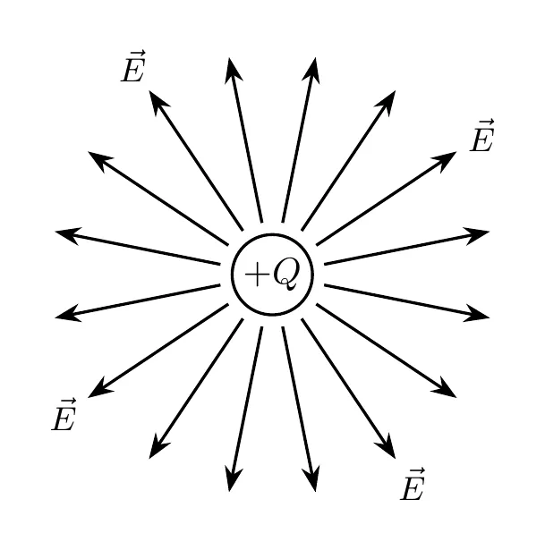
Electric field vectors point away from positive charges.

Fields from Negative Charges

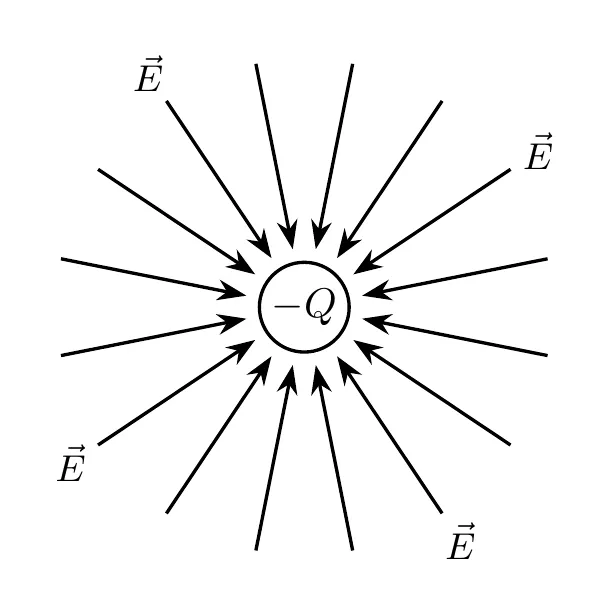
Electric field vectors point toward negative charges.

Why This Convention?

The direction is defined by what would happen to a positive test charge placed there: - Near a positive source, a positive test charge gets pushed away, so the field points outward. - Near a negative source, a positive test charge gets pulled in, so the field points inward.

The fundamental rule stays the same: opposites attract, likes repel.

Test Charges: Positive vs. Negative

Positive Test Charge

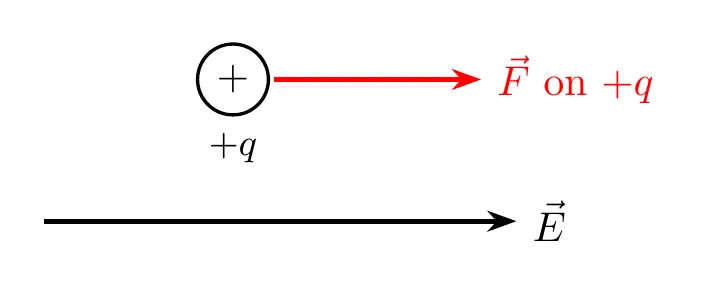
For a positive test charge, the electric force acts in the same direction as the field:

\vec{F}_e = (+q)\vec{E}

Negative Test Charge

For a negative test charge, the electric force acts opposite to the field direction:

\vec{F}_e = (-q)\vec{E}

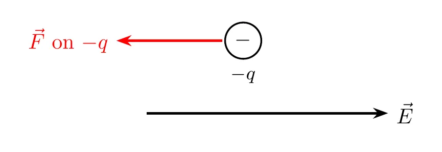
The critical point: the field direction is always defined by the force a positive charge would feel, no matter what charge you’re actually analyzing.

Representing Electric Fields

The electric field is a vector: at every point in space it has a size and a direction.

Superposition of Fields

When several charges are nearby, the net electric field at a point is the vector sum of the fields each charge makes on its own:

\vec{E}_{net} = \vec{E}_1 + \vec{E}_2 + \vec{E}_3 + \cdots

Find each field’s size with

E = k|q|/r^2

, give it a direction (away from positive charges, toward negative ones), then add the components. Example Problem 3 below works one out.

Vector Field Maps

A vector field map draws an arrow at each point on a grid. The arrow points in the direction of the field there, and its length shows how strong the field is.

Field Line Diagrams

A field line diagram is a simplified version of a vector field map. Instead of separate arrows, it draws continuous lines that follow the field. The rules: - Field lines start on positive charges and end on negative charges. Lines from a lone charge run off to (or come in from) infinity. - The field at any point is tangent to the field line through that point, pointing the way the line’s arrows go. - Where the lines are close together, the field is strong. Where they spread apart, it’s weak. - The number of lines leaving or entering a charge is proportional to the size of the charge. - Field lines never cross, since the field can only point one way at each point.

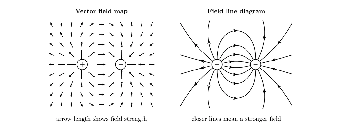
Both diagrams show the same pair of equal and opposite charges (a dipole). Between the charges, the field points from

+

-

. It’s strongest right next to each charge, where the map’s arrows are longest and the lines are most crowded.

A field line is not the path a charge follows. A charge’s acceleration points along the field (or opposite it, for a negative charge), but its velocity can point some other way.

Conductors vs. Insulators

Understanding material properties is essential for any electrostatics analysis.

Conductors

Definition: materials that let electric charge (electrons) flow freely.

Characteristics: - The mobile charge carriers can move all through the material. - Common examples: metals like copper, aluminum, silver, and gold. - Excess charge spreads out on the outer surface.

Insulators

Definition: materials that don’t let electric charge flow freely.

Characteristics: - The charges stay more or less fixed in place. - Common examples: rubber, plastic, glass, wood, styrofoam. - Excess charge stays spread through the volume.

Electrostatic Equilibrium

Electrostatic equilibrium is when there’s no net motion of charge inside a material. The keyword is “static,” meaning no continuous flow (no current), though the charges may shift around initially to get there.

Insulators in Equilibrium

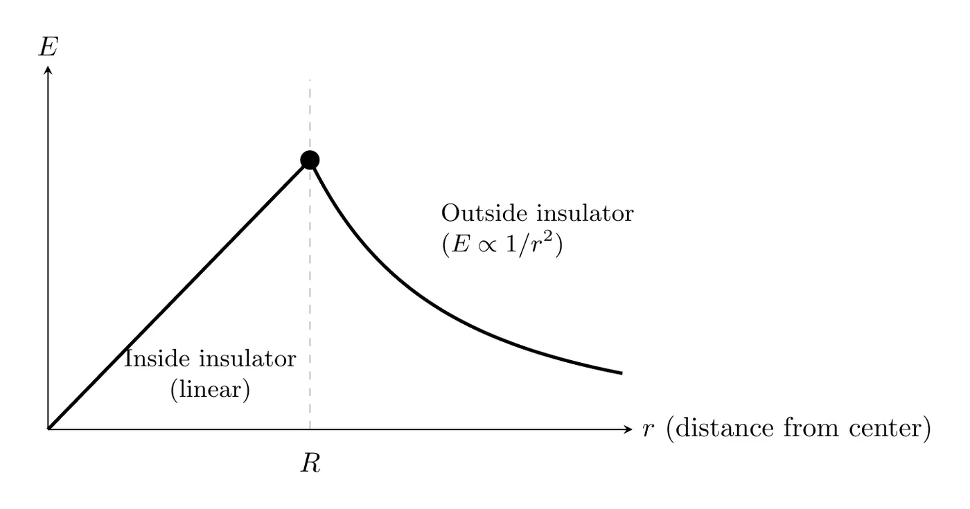
When an insulator reaches electrostatic equilibrium:

Charge distribution: the excess charge can sit anywhere in the volume, inside as well as on the surface. Charges can’t move through an insulator, so they stay wherever they were put. (Problems usually tell you how, such as “spread uniformly through the volume.”)

Electric field: a field exists both inside and outside the insulator.

Field behavior:

Inside: for a sphere with its charge spread uniformly through its volume, the field increases linearly with distance from the center ( $E = kQr/R^3$ , derived in Topic 1.6). Other charge arrangements give other shapes inside.

Outside: the field follows the inverse square law.

Conductors in Equilibrium

When a conductor reaches electrostatic equilibrium:

Charge distribution: all the excess charge sits on the surface only, and the interior has no net charge.

Field inside: $E_{inside} = 0$ , always.

Field at the surface: the field is perpendicular to the surface.

Field outside: it follows the same inverse square law as an insulator.

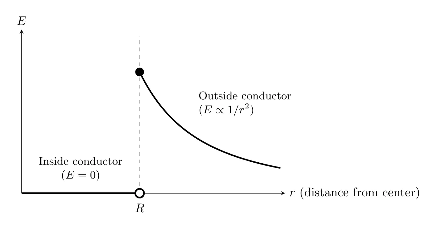
The critical difference: conductors have zero internal field, while insulators have a non-zero internal field.

Why Is the Field Zero Inside a Conductor?

In a conductor, the charges are free to move. Any internal field would push them around until that field got canceled out. Equilibrium is only reached once the internal field hits zero.

The same idea explains why the field just outside a conductor is perpendicular to its surface. If the field had a piece running along the surface, it would push the surface charges sideways and they’d keep moving. Once the charges stop moving, that piece has to be zero, so whatever field is left points straight out of (or into) the surface. Topic 3.1 goes further with conductors.

Electric Field Outside Charged Objects

For a charged sphere, conducting or insulating, as long as its charge is spread symmetrically around the center, the field outside the surface (at

r > R

) follows:

E = k\frac{Q}{r^2}

where: -

E

= field magnitude (N/C) -

k

= Coulomb’s constant (

9 \times 10^9

N·m²/C²) -

Q

= total charge on the object (C) -

r

= distance from the center (m)

Deriving It

Start with Coulomb’s Law:

F_e = k\frac{Qq}{r^2}

where

Q

is the source charge and

q

is a test charge.

Using the definition

E = \frac{F_e}{q}

E = \frac{k\frac{Qq}{r^2}}{q} = k\frac{Q}{r^2}

The test charge cancels out, leaving just the field from the source charge

Q

Example Problem 1: Field from the Force on an Electron

Given: an electron feels an eastward force of

4.80 \times 10^{-17}

N in an electric field.

Find: (a) The electric field (magnitude and direction). (b) The force a proton would feel in that same field.

Solution

Part (a): the electric field

Use the field definition:

E = \frac{F_e}{|q|}

The electron’s charge magnitude is

|q_e| = 1.6 \times 10^{-19}

E = \frac{4.80 \times 10^{-17}}{1.6 \times 10^{-19}} = 300 \text{ N/C}

Direction: the electron is negative and feels an eastward force. Since negative charges feel a force opposite to the field, the field points west.

Answer (a):

E = 300

N/C, directed west.

Part (b): the force on a proton

The proton has the same charge magnitude,

|q_p| = 1.6 \times 10^{-19}

F_e = qE = (1.6 \times 10^{-19})(300) = 4.80 \times 10^{-17} \text{ N}

Direction: the proton is positive, so it feels a force in the same direction as the field, which is west.

Answer (b):

F = 4.80 \times 10^{-17}

N, directed west.

Example Problem 2: Equilibrium Field Analysis

Given: a particle with charge

q_1 = +2.0 \times 10^{-8}

C feels an upward force of

4.0 \times 10^{-6}

N at a point in an electric field.

Find: (a) The electric field at that point. (b) If a charge

q_2 = -1.0 \times 10^{-8}

C is placed there instead, what force does it feel? (c) How far is this point from a source charge

Q = +2.0 \times 10^{-8}

C creating the field?

Solution

Part (a): the electric field

E = \frac{F_e}{q} = \frac{4.0 \times 10^{-6}}{2.0 \times 10^{-8}} = 200 \text{ N/C}

Direction: the positive charge feels an upward force, so the field points upward.

Answer (a):

E = 200

N/C, upward.

Part (b): the force on the negative charge

F_e = q_2 E = (-1.0 \times 10^{-8})(200) = -2.0 \times 10^{-6} \text{ N}

Direction: the negative sign means it’s opposite the field, so downward.

Answer (b):

F = 2.0 \times 10^{-6}

N, downward.

Part (c): the distance from the source

Using

E = k\frac{Q}{r^2}

, solve for

r

r = \sqrt{\frac{kQ}{E}}

r = \sqrt{\frac{(9 \times 10^9)(2.0 \times 10^{-8})}{200}}

r = \sqrt{\frac{180}{200}} = \sqrt{0.9} = 0.949 \text{ m}

Answer (c):

r \approx 0.95

Example Problem 3: Net Field from Two Charges

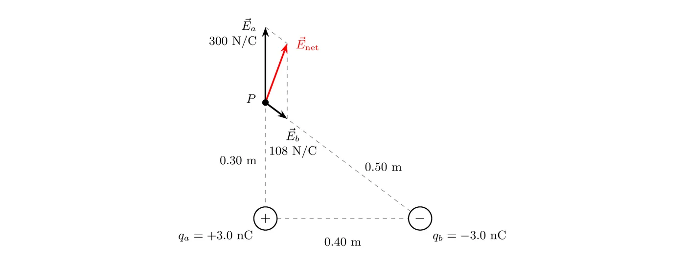
Given:

q_a = +3.0

nC sits at the origin and

q_b = -3.0

nC sits on the x-axis at

x = 0.40

m. Point P is on the y-axis at

y = 0.30

Find: (a) The net electric field at P (magnitude and direction). (b) The force on an electron placed at P.

Solution

Step 1: Field from the positive charge

P is 0.30 m straight above

q_a

. The field points away from a positive charge, so it points straight up (

+y

E_a = k\frac{|q_a|}{r_a^2} = (9.0 \times 10^9\text{ N·m}^2\text{/C}^2)\frac{3.0 \times 10^{-9} \text{ C}}{(0.30 \text{ m})^2} = 300 \text{ N/C}

Step 2: Field from the negative charge

The distance from

q_b

to P is

\sqrt{(0.40 \text{ m})^2 + (0.30 \text{ m})^2} = 0.50

m. The field points toward a negative charge, so it points from P toward

q_b

: down and to the right.

E_b = (9.0 \times 10^9\text{ N·m}^2\text{/C}^2)\frac{3.0 \times 10^{-9} \text{ C}}{(0.50 \text{ m})^2} = 108 \text{ N/C}

Step 3: Break the second field into components

Going from P to

q_b

is 0.40 m to the right and 0.30 m down, over a distance of 0.50 m:

E_{b,x} = (108 \text{ N/C})\frac{0.40}{0.50} = 86.4 \text{ N/C} \qquad E_{b,y} = -(108 \text{ N/C})\frac{0.30}{0.50} = -64.8 \text{ N/C}

Step 4: Add the components

E_x = 0 + 86.4 = 86.4 \text{ N/C} \qquad E_y = 300 - 64.8 = 235.2 \text{ N/C}

E_{net} = \sqrt{(86.4)^2 + (235.2)^2} = 2.5 \times 10^2 \text{ N/C}

\theta = \tan^{-1}\left(\frac{235.2}{86.4}\right) = 70^\circ \text{ above the } +x \text{ axis}

Answer (a):

E_{net} = 2.5 \times 10^2

N/C, pointing

70°

above the

+x

axis (up and a bit to the right).

Step 5: The force on an electron

The electron is negative, so the force points opposite the field:

70°

below the

-x

axis (down and a bit to the left).

F = |q|E = (1.60 \times 10^{-19} \text{ C})(2.5 \times 10^2 \text{ N/C}) = 4.0 \times 10^{-17} \text{ N}

Answer (b):

4.0 \times 10^{-17}

N, directed

70°

below the

-x

axis.

Example Problem 4: Conducting vs. Insulating Sphere

Given: two spheres, each with radius

R = 0.10

m and charge

Q = +5.0

nC. Sphere 1 is metal (a conductor). Sphere 2 is plastic (an insulator) with its charge spread uniformly through its volume.

Find: the field of each sphere at

r = 0.060

m (inside),

r = 0.10

m (at the surface), and

r = 0.20

m (outside).

Solution

Inside, at 0.060 m: - Metal sphere:

E = 0

. Its charge sits on the surface, and the field inside a conductor in equilibrium is zero. - Plastic sphere: the field grows linearly inside,

E = kQr/R^3

(Topic 1.6 derives this):

E = \frac{kQr}{R^3} = \frac{(9.0 \times 10^9\text{ N·m}^2\text{/C}^2)(5.0 \times 10^{-9} \text{ C})(0.060 \text{ m})}{(0.10 \text{ m})^3} = 2.7 \times 10^3 \text{ N/C}

At the surface, 0.10 m: from here outward, both spheres act like a point charge at their centers:

E = \frac{kQ}{R^2} = \frac{(9.0 \times 10^9\text{ N·m}^2\text{/C}^2)(5.0 \times 10^{-9} \text{ C})}{(0.10 \text{ m})^2} = 4.5 \times 10^3 \text{ N/C}

Outside, at 0.20 m: the same formula for both spheres:

E = \frac{(9.0 \times 10^9\text{ N·m}^2\text{/C}^2)(5.0 \times 10^{-9} \text{ C})}{(0.20 \text{ m})^2} = 1.1 \times 10^3 \text{ N/C}

The read: outside, you can’t tell the spheres apart. Inside, the metal sphere’s field is zero while the plastic sphere’s isn’t. Doubling the distance from 0.10 m to 0.20 m cut the field to 1/4, from

4.5 \times 10^3

to about

1.1 \times 10^3

N/C.

Common Mistakes

Confusing the force direction with the field direction for negative charges. Negative charges feel a force opposite to the field. Always account for the sign.

Assuming conductors and insulators behave the same. The interior field is zero for conductors but non-zero for insulators. That’s a fundamental difference.

Putting charge inside a conductor at equilibrium. All the excess charge on a conductor sits on the surface. The interior has no net charge.

Using the wrong charge in field calculations. When you calculate the field from a force ( $E = F/q$ ), use the charge of the object feeling the force, not the source creating the field.

Forgetting that the exterior fields are identical. Outside the surface, a conducting sphere and an insulating sphere with the same charge (spread symmetrically) both produce a field of $E = kQ/r^2$ , whatever the internal differences. This only works for spheres. For other shapes, the outside field depends on the shape.

Back Next