

1.4 - Electric Fields of Charge Distributions
Introduction to Charge Distributions
So far we’ve looked at fields from point charges. Now we extend that to continuous charge distributions, where the charge is spread over a length, an area, or a volume instead of being concentrated at a point.
These show up on exams a lot as “derive an expression” questions, which means integration and vector analysis.
The General Integration Formula
To find the field from a continuous distribution, use integration paired with the principle of superposition.
The Fundamental Equation
or equivalently:
where:
- = an infinitesimal charge element
- = distance from to the point where you want the field
- = a unit vector pointing from toward the field point
- N·m²/C²
The key concept: you break the charged object into infinitely small pieces, find the field contribution from each piece, then sum (integrate) all of them.
Simplifying with Symmetry
A lot of charge distribution problems get much easier if you spot the symmetry. When symmetric charge elements produce field components that cancel in certain directions, you only have to integrate the components that survive.
The strategy:
1. Identify the symmetry in the charge distribution.
2. Figure out which field components cancel.
3. Integrate only the surviving components.
This cuts down the math dramatically.
Common Charge Distributions
1. Infinite Wire (Line of Charge)
A very long straight wire with uniform charge density, so long that the end effects don’t matter.
Characteristics:
- Assume infinite length, so you can ignore contributions from the ends.
- The high symmetry makes the analysis simpler.
- The field points radially outward from (or inward toward) the wire.
2. Finite Wire (Line Segment)
A straight wire segment with uniform charge density and definite endpoints.
Characteristics:
- You have to account for every part, including near the ends.
- It’s less symmetric than the infinite case.
- The integration limits are more involved.
3. Arc or Semicircle
A curved segment of charge, usually part of a circular path.
Characteristics:
- Could be a full semicircle (180°) or a partial arc, like a 90° quarter-circle.
- The angular symmetry often simplifies things.
- Angular coordinates are the natural choice.
4. Ring of Charge
A complete circular loop with uniform charge distribution.
Characteristics:
- High rotational symmetry.
- You’re usually asked for the field along the axis perpendicular to the ring’s plane.
- The components perpendicular to the axis cancel by symmetry.
Detailed Example: Ring of Charge
Problem: Derive an expression for the electric field at a point P on the axis of a uniformly charged ring. The ring has radius and total charge . Point P sits a distance from the ring’s center along the axis.
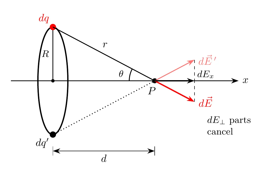
Setup and Symmetry Analysis
The key constants:
- Ring radius: , the same for every charge element.
- Distance to P: , measured along the axis.
- Distance from any ring element to P: , which is also constant.
The symmetry observation: every charge element on the ring is the same distance from point P. For any element on one side of the ring, there’s a matching element on the opposite side. Their field contributions have:
- Components perpendicular to the axis that cancel.
- Components parallel to the axis that add.
So the net field points along the axis only: .
The Derivation
Step 1: Express the axial component
Each infinitesimal element produces a field:
The axial component is:
Step 2: Find the geometric relations
From the geometry:
Step 3: Substitute and identify the constants
Step 4: Integrate
Since , , and therefore are all constants (the same for every ), factor them out:
The integral of over the whole ring is just the total charge :
The final expression:
or equivalently:
The field points along the axis, away from the ring if and toward it if .
Checking the Limiting Cases
Good physics practice: verify that your expression makes sense in the extreme cases.
Case 1: At the center ()
That makes sense. By symmetry, all the field contributions cancel at the center.
Case 2: Very far from the ring ()
That’s the field of a point charge. From far away, the ring just looks like a point.
Case 3: Where the field is strongest
Taking the derivative and setting it to zero shows the maximum happens at .
Putting In Numbers
A ring of radius m carries nC. At m from its center along the axis:
The strongest field on the axis is at m, where N/C. The graph shows the whole axis, with measured from the ring’s center (negative is the other side of the ring):
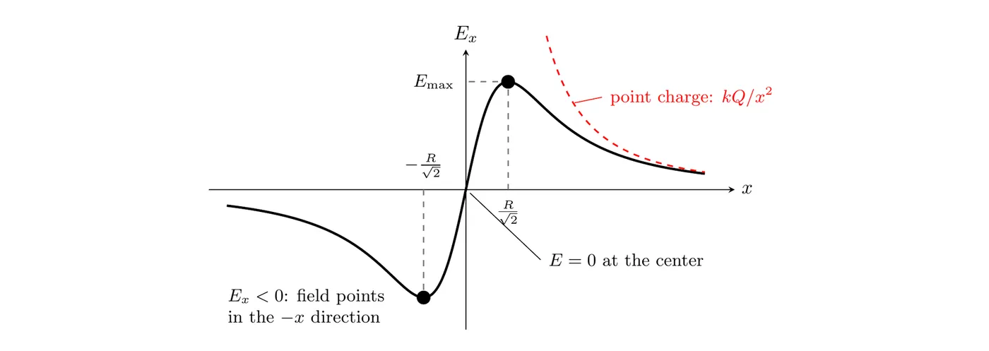
How to read it:
- at the center, rises to a maximum at , then falls off.
- Far from the ring, the curve merges with the point charge curve (red, dashed).
- On the other side of the ring (), the field has the same strength but points the other way, in the direction, so is negative.
Alternative Example: Charged Rod Along the Axis
Problem: A thin rod of length has uniform charge density . Find the electric field at a point P on the rod’s axis, a distance from the nearest end.
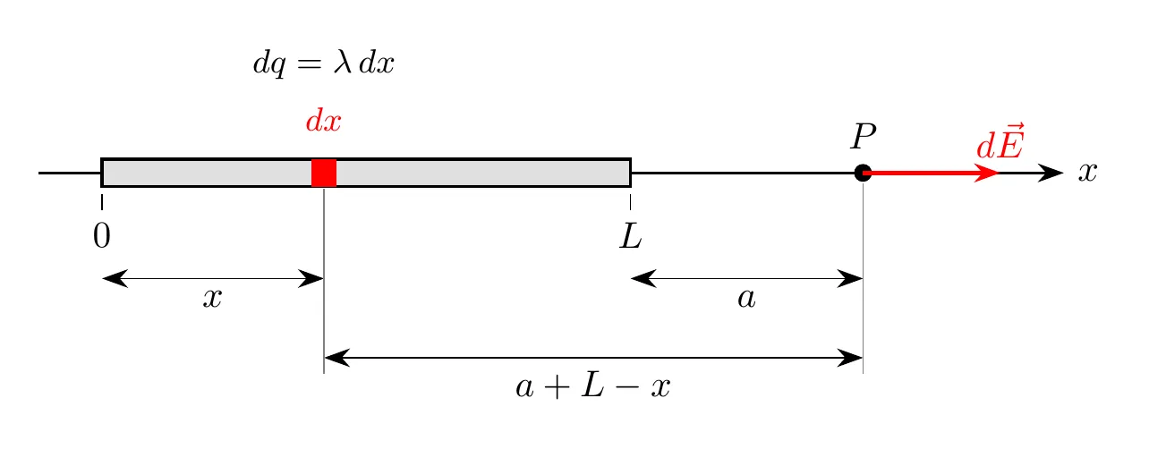
Solution
Step 1: Set up the integral
Each element carries charge and sits a distance from P:
Every contribution points the same way (along the axis), so:
Step 2: Integrate
Factor out the constants:
Use the substitution , so .
When : .
When : .
Since the total charge is :
Finite Line of Charge: Point on the Perpendicular Bisector
Problem: A thin rod of length carries charge spread uniformly, so . Find the electric field at point P, a distance from the rod’s midpoint along the perpendicular bisector.
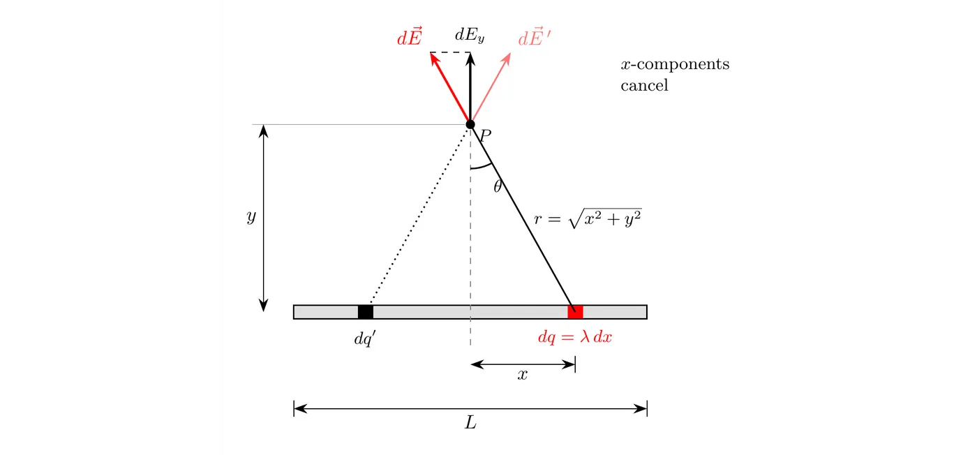
Setup and Symmetry Analysis
Put the rod on the x-axis from to , with P on the y-axis. A small piece at position carries and sits a distance from P.
The symmetry observation: for every piece at there’s a matching piece at . Their x-components cancel and their y-components add, so the net field points straight along the bisector: .
The Derivation
Step 1: Express the y-component
With measured from the bisector, :
Step 2: Set up the integral
This time changes from piece to piece, so it stays inside the integral. Only , , and are constants:
Step 3: Integrate
The substitution turns the integrand into , which gives this standard result (you can check it by differentiating the right side):
Since :
The field points along the bisector, away from the rod if and toward it if .
Checking the Limiting Cases
Far from the rod (y much bigger than L): , so , the field of a point charge.
Very long rod (L much bigger than y): , so . That’s the field of an infinite line (next section).
Putting In Numbers
A rod of length 0.40 m carries 6.0 nC spread uniformly. At 0.15 m from its midpoint, on the perpendicular bisector:
Infinite Line of Charge
Let the rod in the last section get infinitely long. The limits become to , and the bracket from Step 3 becomes , so , matching the very long rod check above. Writing for the distance from the line, and using :
The field points straight out from the line (straight in if ) and falls off as . That’s slower than a point charge’s , because the line’s charge keeps going in both directions forever: doubling your distance only cuts the field in half.
Long cylinders: outside a long, uniformly charged cylinder, the field is the same, with equal to the cylinder’s charge per unit length. Topic 1.6 gets this much faster with Gauss’s Law and finds the field inside the cylinder too.
Semicircular Arc: Field at the Center
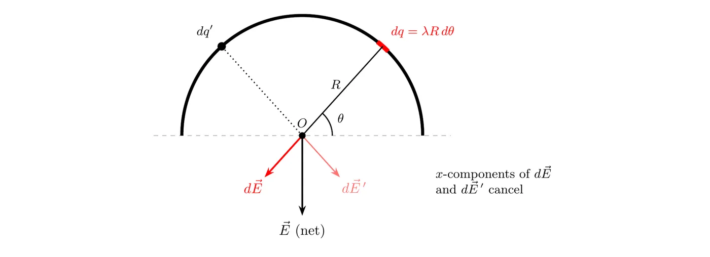
Problem: A thin rod bent into a semicircle of radius carries charge spread uniformly. Find the electric field at the center of the circle, point O.
Setup and Symmetry Analysis
Measure the angle around the arc from the axis, so the arc runs from to . The arc’s length is , so . A small piece of arc has length and charge .
Every piece is the same distance from O. The pieces at and are mirror images, so their x-components cancel and their y-components add. For positive charge, the net field points straight down, away from the arc.
The Derivation
Step 1: Express the y-component
Step 2: Integrate over the arc
Using :
The field points away from the middle of the arc if , and toward it if . It’s only times the you’d get with all the charge at one point a distance away, because the sideways parts of the pieces’ fields cancel.
Part of an Arc
For an arc that covers only part of the semicircle, use the same setup with different limits. The components may not cancel anymore, so integrate both. For a quarter circle from to :
Both components have size , so , pointing along the line, straight away from the midpoint of the arc (toward the lower left if ). For a quarter circle, .
Problem-Solving Strategy
- Draw a clear diagram with the charge distribution, the field point, and your coordinates.
- Identify the symmetry. Which components cancel?
- Choose your coordinate system so the axes line up with the symmetry.
- Express in terms of your integration variable:
- Linear:
- Surface:
- Volume:
- Express the distance from to the field point in terms of your integration variable.
- Set up the integral with the right limits.
- Identify the constants and factor them out before integrating.
- Check the limiting cases to make sure the answer makes physical sense.
Common Mistakes
- Forgetting the geometric factors like cosθ or sinθ. When you find field components, you have to project with trig functions. Skipping them gives you the wrong vector directions.
- Treating variable distances as constants. Make sure you correctly express how the distance from each charge element to P changes across the distribution. Only factor out things that are genuinely constant.
- Setting up the wrong integration limits. Define your coordinate system carefully and figure out where the charge distribution starts and ends in it.
- Not exploiting symmetry. A lot of problems get much harder if you don’t notice that certain components cancel. Always look for symmetry before you integrate.
- Forgetting that electric field is a vector. You have to integrate the components separately, not just the magnitudes. Use unit vectors or component notation consistently.