1.2 - Displacement, Velocity, and Acceleration

The Object Model

When you analyze motion, you ignore size, shape, and internal structure. A car gets treated as a single object, with all its moving parts set aside. A ball becomes a point mass. This simplification lets you focus on the motion itself.

The object still keeps its mass (and its charge, if it has one). Only the size, shape, and inner parts are ignored. This works as long as you only care about where the object goes, not how it spins or bends. A spinning wheel can’t be treated as a single point, which is why rotation gets its own units later in the course.

Displacement

Displacement is the change in an object’s position.

\Delta x = x_f - x_0

where: -

\Delta x

= displacement -

x_f

= final position -

x_0

= initial position

Displacement is a vector that describes the change in position, not the total distance traveled.

In two or three dimensions, displacement is the change in the position vector:

\Delta\vec{r} = \vec{r} - \vec{r}_0

Distance vs. displacement: distance is the total length of the path (a scalar, never negative). Displacement only compares the start and the end. A runner who goes once around a 400 m track covers a distance of 400 m but has a displacement of zero.

Average Velocity and Acceleration

Average Velocity

Average velocity is the change in position over time across an interval.

v_{avg} = \frac{\Delta x}{\Delta t} = \frac{x_f - x_0}{t_f - t_0}

Graphically, this is the slope of a position-time graph between two points.

As a vector, average velocity is

\vec{v}_{avg} = \frac{\Delta\vec{r}}{\Delta t}

, and it points in the same direction as the displacement.

Only the start and the end matter. Averages are calculated from the initial and final states, so anything that happens in between (speeding up, stopping, turning around) doesn’t change the answer. That’s also why average speed (total distance divided by time) can be bigger than the size of the average velocity: distance counts every back-and-forth, but displacement doesn’t.

Average Acceleration

Average acceleration is the change in velocity over time across an interval.

a_{avg} = \frac{\Delta v}{\Delta t} = \frac{v_f - v_0}{t_f - t_0}

Graphically, this is the slope of a velocity-time graph between two points.

Example: a tennis ball hits a wall at 15 m/s and bounces straight back at 12 m/s. It’s in contact with the wall for 0.0050 s. Taking the ball’s incoming direction as positive:

a_{avg} = \frac{v_f - v_0}{\Delta t} = \frac{(-12) - (+15)}{0.0050} = -5.4 \times 10^3 \text{ m/s}^2

The change in velocity is

-27

m/s, not

-3

m/s. Reversing direction means the ball loses all 15 m/s and then gains 12 m/s the other way.

What counts as accelerating: an object is accelerating whenever its velocity changes in magnitude, direction, or both. A car going around a curve at a steady 15 m/s is accelerating, because the direction of its velocity keeps changing.

Speeding up or slowing down? Compare the signs of velocity and acceleration: - Same sign: speeding up. - Opposite signs: slowing down. A negative acceleration does not automatically mean slowing down. A car moving in the

-x

direction with a negative acceleration is speeding up.

Instantaneous Velocity and Acceleration

Here’s a key distinction: in calculus-based physics, the acceleration may or may not be constant. That means you need derivatives and integrals instead of just assuming constant acceleration.

As the time interval shrinks toward zero (

\Delta t \to 0

), the average values turn into instantaneous values at a single moment in time.

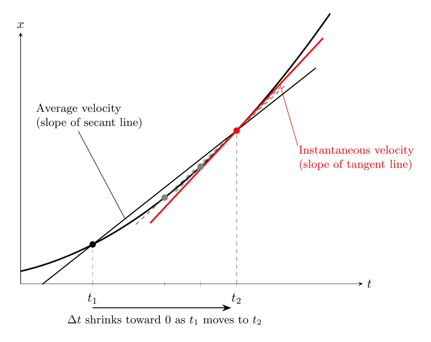
1.2 - Displacement, Velocity, and Acceleration

Seeing it with numbers: take

x(t) = 0.50t^3

(in meters) and find the velocity at

t = 3.0

s by shrinking the time interval:

Interval	$\Delta t$ (s)	Average velocity (m/s)
3.0 s to 4.0 s	1.0	18.5
3.0 s to 3.1 s	0.1	13.955
3.0 s to 3.01 s	0.01	13.545
3.0 s to 3.001 s	0.001	13.5045

The averages close in on 13.5 m/s. Calculus gets there directly:

v = \frac{dx}{dt} = 1.5t^2

, and

1.5(3.0)^2 = 13.5

m/s. That’s the instantaneous velocity at

t = 3.0

Instantaneous Velocity

v = \frac{dx}{dt}

Velocity is the derivative of position with respect to time.

Instantaneous Acceleration

a = \frac{dv}{dt}

Acceleration is the derivative of velocity with respect to time.

Both work for vectors too:

\vec{v} = \frac{d\vec{r}}{dt}

and

\vec{a} = \frac{d\vec{v}}{dt}

. In two or three dimensions, take the derivative of each component separately (see 1.5).

Heads up:

v = \frac{dx}{dt}

and

a = \frac{dv}{dt}

are not printed on the AP Physics C equation sheet. The sheet only lists the integral versions,

\Delta x = \int v_x(t)\,dt

and

\Delta v_x = \int a_x(t)\,dt

, so know the derivative forms by heart.

How Position, Velocity, and Acceleration Connect

Going Down with Differentiation

\text{Position} \xrightarrow{\text{derivative}} \text{Velocity} \xrightarrow{\text{derivative}} \text{Acceleration}

x(t) \xrightarrow{\frac{d}{dt}} v(t) \xrightarrow{\frac{d}{dt}} a(t)

Going Up with Integration

Integration is the anti-derivative, which lets you work backwards.

\text{Acceleration} \xrightarrow{\text{integrate}} \text{Velocity} \xrightarrow{\text{integrate}} \text{Position}

Finding velocity from acceleration:

Start with

a = \frac{dv}{dt}

Multiply both sides by

dt

dv = a \, dt

Integrate both sides:

\int dv = \int a \, dt

v(t) = \int a(t) \, dt + v_0

where

v_0

is the constant of integration (the initial velocity).

Finding position from velocity:

Start with

v = \frac{dx}{dt}

Multiply both sides by

dt

dx = v \, dt

Integrate both sides:

\int dx = \int v \, dt

x(t) = \int v(t) \, dt + x_0

where

x_0

is the constant of integration (the initial position).

Shortcut with definite integrals: if you integrate from

t = 0

to a later time

t

, the starting value shows up on its own, with no

+C

to solve for (

t'

is just the variable you integrate over):

v(t) = v_0 + \int_0^t a(t')\,dt' \qquad x(t) = x_0 + \int_0^t v(t')\,dt'

These are the equation sheet’s

\Delta v_x = \int a_x(t)\,dt

and

\Delta x = \int v_x(t)\,dt

with the starting values added back. For the example below,

v(t) = -15 + \int_0^t 24t'\,dt' = 12t^2 - 15

, the same answer.

Finding the Constants of Integration

You pin down the constants (

v_0

x_0

) using the initial conditions the problem gives you. These usually tell you: - The position at

t = 0

: “at

t = 0

x = x_0

.” - The velocity at

t = 0

: “at

t = 0

v = v_0

.”

Example Problem

Problem: A particle moves along the x-axis with acceleration

a(t) = 24t

(in m/s²). At

t = 0

, the particle is at the origin with a velocity of

-15

m/s. Where is it at

t = 3

seconds?

Step 1: Find the Velocity Function

Given:

a(t) = 24t

Since

a = \frac{dv}{dt}

, integrate to get velocity:

v(t) = \int a(t) \, dt = \int 24t \, dt

Using the power rule,

\int t^n \, dt = \frac{t^{n+1}}{n+1} + C

v(t) = 24 \cdot \frac{t^2}{2} + C = 12t^2 + C

Apply the initial condition, that at

t = 0

v = -15

m/s:

v(0) = 12(0)^2 + C = -15

C = -15

So:

v(t) = 12t^2 - 15

Step 2: Find the Position Function

Since

v = \frac{dx}{dt}

, integrate to get position:

x(t) = \int v(t) \, dt = \int (12t^2 - 15) \, dt

x(t) = 12 \cdot \frac{t^3}{3} - 15t + C

x(t) = 4t^3 - 15t + C

Apply the initial condition, that at

t = 0

x = 0

(at the origin):

x(0) = 4(0)^3 - 15(0) + C = 0

C = 0

So:

x(t) = 4t^3 - 15t

Step 3: Find the Position at t = 3 seconds

x(3) = 4(3)^3 - 15(3)

x(3) = 4(27) - 45

x(3) = 108 - 45

x(3) = 63 \text{ m}

Answer: the particle is at 63 m at

t = 3

seconds.

The physical read: even though the particle starts out moving in the negative direction (negative velocity), the positive acceleration slows it down, stops it, and then pushes it in the positive direction, landing it at a positive final position.

Example Problem: Going Down with Derivatives

Problem: a particle moves along the x-axis with position

x(t) = 2.0t^3 - 9.0t^2 + 12t

(in meters, with

t

in seconds).

Find $v(t)$ and $a(t)$ .

When is the particle at rest?

At $t = 2.5$ s, is it speeding up or slowing down?

Find its displacement, total distance, average velocity, and average speed from $t = 0$ to $t = 3.0$ s.

Part (a): Velocity and Acceleration Functions

Differentiate once for velocity and again for acceleration:

v(t) = \frac{dx}{dt} = 6.0t^2 - 18t + 12

a(t) = \frac{dv}{dt} = 12t - 18

Part (b): When Is It at Rest?

Set

v = 0

and factor:

6.0(t^2 - 3t + 2) = 6.0(t - 1)(t - 2) = 0

Answer: the particle is at rest at

t = 1.0

s and

t = 2.0

s. These are turnaround points, since

v

changes sign at each one. Being at rest for an instant doesn’t mean

a = 0

: at

t = 1.0

a = 12(1.0) - 18 = -6.0

m/s².

Part (c): Speeding Up or Slowing Down at t = 2.5 s

v(2.5) = 6.0(2.5)^2 - 18(2.5) + 12 = 4.5 \text{ m/s}

a(2.5) = 12(2.5) - 18 = 12 \text{ m/s}^2

Answer: both are positive (same sign), so the particle is speeding up.

Part (d): Displacement, Distance, and Averages

Find the position at the start, at each turnaround, and at the end:

x(0) = 0 \qquad x(1.0) = 5.0 \text{ m} \qquad x(2.0) = 4.0 \text{ m} \qquad x(3.0) = 9.0 \text{ m}

Displacement only compares the start and the end:

\Delta x = 9.0 - 0 = 9.0

Distance adds up every leg, ignoring direction: forward 5.0 m, back 1.0 m, then forward 5.0 m, for a total of 11 m.

v_{avg} = \frac{\Delta x}{\Delta t} = \frac{9.0}{3.0} = 3.0 \text{ m/s} \qquad \text{average speed} = \frac{11}{3.0} = 3.7 \text{ m/s}

The read: the average speed is bigger than the average velocity because the particle backtracked between

t = 1.0

s and

t = 2.0

Integration Rules Summary

Power rule:

\int t^n \, dt = \frac{t^{n+1}}{n+1} + C \quad (n \neq -1)

Constant multiple rule:

\int k \cdot f(t) \, dt = k \int f(t) \, dt

Sum/difference rule:

\int [f(t) \pm g(t)] \, dt = \int f(t) \, dt \pm \int g(t) \, dt

Common Mistakes

Forgetting the constant of integration. Always include $+ C$ when you integrate, then use the initial conditions to solve for it.

Not applying initial conditions correctly. Substitute $t = 0$ (or whatever time is given) into your integrated function and set it equal to the given initial value.

Confusing average and instantaneous values. Average quantities use $\Delta$ notation and cover an interval. Instantaneous quantities use derivatives and are evaluated at a single instant.

Applying the power rule wrong. Add 1 to the exponent and divide by the new exponent: $\int t^2 \, dt = \frac{t^3}{3}$ , not $\frac{t^3}{2}$ .

Assuming constant acceleration. In calculus-based physics, acceleration can be a function of time. Work from the given function, not from kinematic equations that assume constant acceleration.

Sign errors with negative initial conditions. Watch the negatives. If $v_0 = -15$ m/s, then $C = -15$ , so your velocity function includes $-15$ , not $+15$ .

Mixing up distance and displacement. If the velocity changes sign during the interval, the object turned around. Split the interval at each turnaround to find the distance. Displacement only needs the start and the end.

Back Next