1.3 - Representing Motion

Ways to Represent Motion

You can represent motion in several ways: - Diagrams and figures. - Graphs. - Equations. - Narrative descriptions. - Data tables.

In physics, graphs and equations are the ones you’ll use most.

Motion Diagrams

Motion diagrams show a series of dots marking an object’s position at equal time intervals. You can turn these into data tables, which then become graphs.

Reading a motion diagram: - Equal spacing between dots: constant velocity. - Spacing getting bigger: speeding up. - Spacing getting smaller: slowing down.

Velocity arrows drawn at each dot get longer as the object speeds up. The acceleration arrow points the way the velocity is changing: the same direction as the motion when speeding up, and the opposite direction when slowing down.

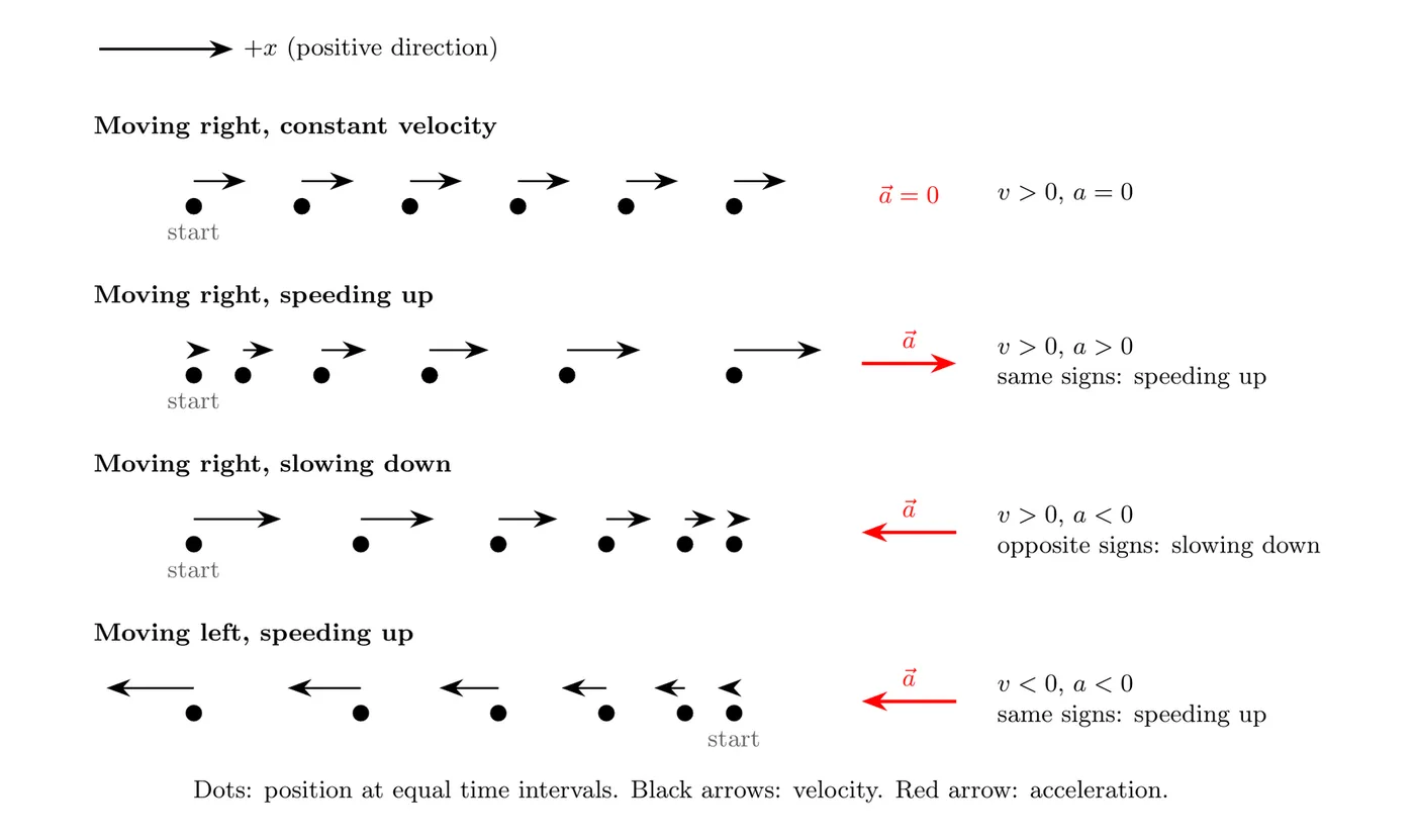
The bottom two rows both have negative acceleration, but one is slowing down and the other is speeding up. The sign of

a

alone doesn’t tell you. Compare it with the sign of

v

Constant vs. Non-Constant Acceleration

Constant Acceleration (Algebra-Based Physics)

In algebra-based courses, you assume constant acceleration and use the kinematic equations:

v = v_0 + at

x = x_0 + v_0 t + \frac{1}{2}at^2

v^2 = v_0^2 + 2a(x - x_0)

x = x_0 + \frac{1}{2}(v_0 + v)t

These only work when the acceleration is constant.

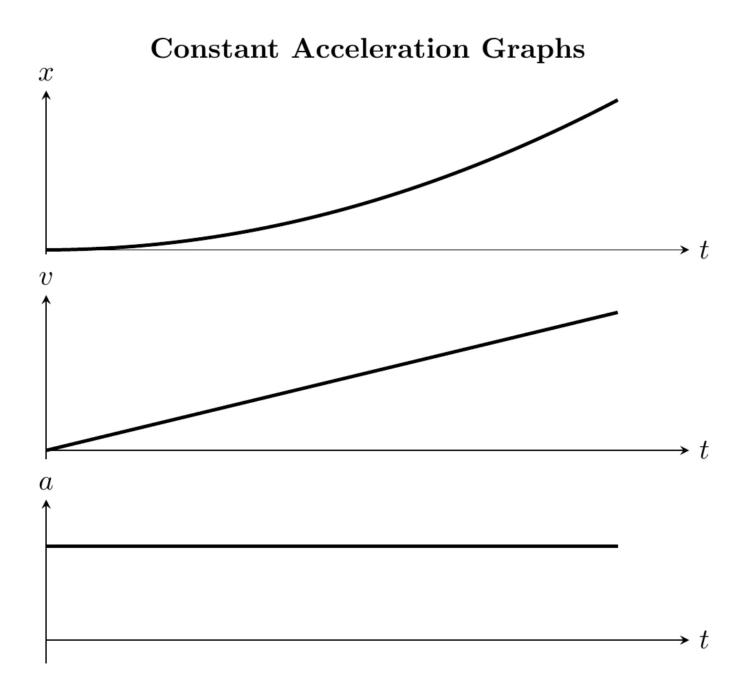
The first three are on the AP Physics C equation sheet too, written for motion along

x

(for example,

v_x = v_{x0} + a_x t

). They work in any single direction (swap

x

for

y

for vertical motion), and you’ll use them all the time in Physics C whenever the acceleration is constant: free fall, projectiles, and anything with a constant net force. The fourth one,

x = x_0 + \frac{1}{2}(v_0 + v)t

, isn’t on the sheet, but you can get it by combining the first two.

Where They Come From

Start with a constant acceleration

a

and integrate twice (with

v = v_0

and

x = x_0

t = 0

v = v_0 + \int_0^t a\,dt' = v_0 + at

x = x_0 + \int_0^t (v_0 + at')\,dt' = x_0 + v_0 t + \frac{1}{2}at^2

Solving the first equation for

t = \frac{v - v_0}{a}

and substituting it into the second gives

v^2 = v_0^2 + 2a(x - x_0)

, the one equation without time in it.

Picking an equation: list what you know and what you want. Each equation leaves out one variable. If time isn’t given or asked for, use

v^2 = v_0^2 + 2a(x - x_0)

Example: Stopping Distance

A car moving at 20 m/s brakes at

-5.0

m/s². Time isn’t given, so use the timeless equation with

v = 0

\Delta x = \frac{-v_0^2}{2a} = \frac{-(20)^2}{2(-5.0)} = 40

m. At 40 m/s, the same braking takes

\frac{-(40)^2}{2(-5.0)} = 160

m. Stopping distance is proportional to

v_0^2

, so doubling your speed quadruples your braking distance.

Non-Constant Acceleration (Calculus-Based Physics)

In calculus-based physics, the acceleration can change with time. When it’s not constant, you have to use calculus, and you can’t use the standard kinematic equations.

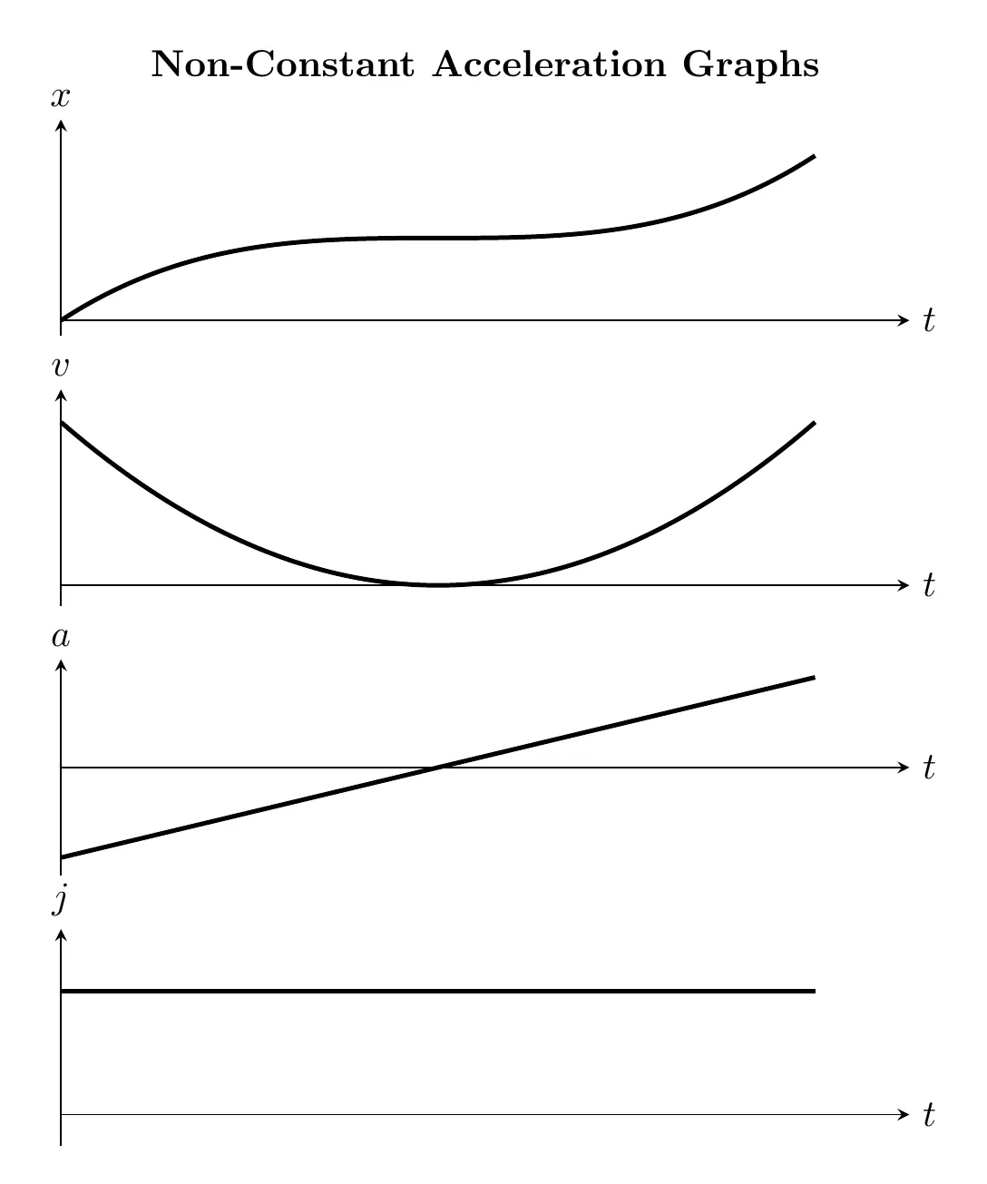
Jerk is the rate of change of acceleration with respect to time:

j = \frac{da}{dt}

When jerk isn’t zero, the acceleration isn’t constant. This is more realistic for real-world motion. For example, driving a car without cruise control means the acceleration is constantly changing. Even with cruise control on, the car may speed up or slow down a bit to hold its set speed over changing terrain.

How the Graphs Relate

The relationships between the position, velocity, and acceleration graphs: - Velocity is the slope of the position-time graph. - Acceleration is the slope of the velocity-time graph. - The area under the velocity-time graph gives displacement. - The area under the acceleration-time graph gives change in velocity.

Slope of a curved graph: when a graph curves, its slope is different at every instant. The instantaneous velocity is the slope of the tangent line to the position-time graph at that point (

v_x = \frac{dx}{dt}

), and the instantaneous acceleration is the slope of the tangent line to the velocity-time graph (

a_x = \frac{dv_x}{dt}

Areas are integrals. These are the equation sheet’s area equations, written with the time limits:

\Delta x = \int_{t_1}^{t_2} v_x(t)\,dt \qquad \Delta v_x = \int_{t_1}^{t_2} a_x(t)\,dt

Area below the time axis counts as negative. On a velocity graph, that’s time spent moving in the negative direction. Add the areas with their signs to get displacement. Add them all as positive numbers to get total distance.

Example: Reading a Velocity Graph

Problem: a cart moves along a straight track, starting from

x = 0

t = 0

. Its velocity-time graph is the middle graph below. The top and bottom graphs show what we’ll work out: its position and its acceleration.

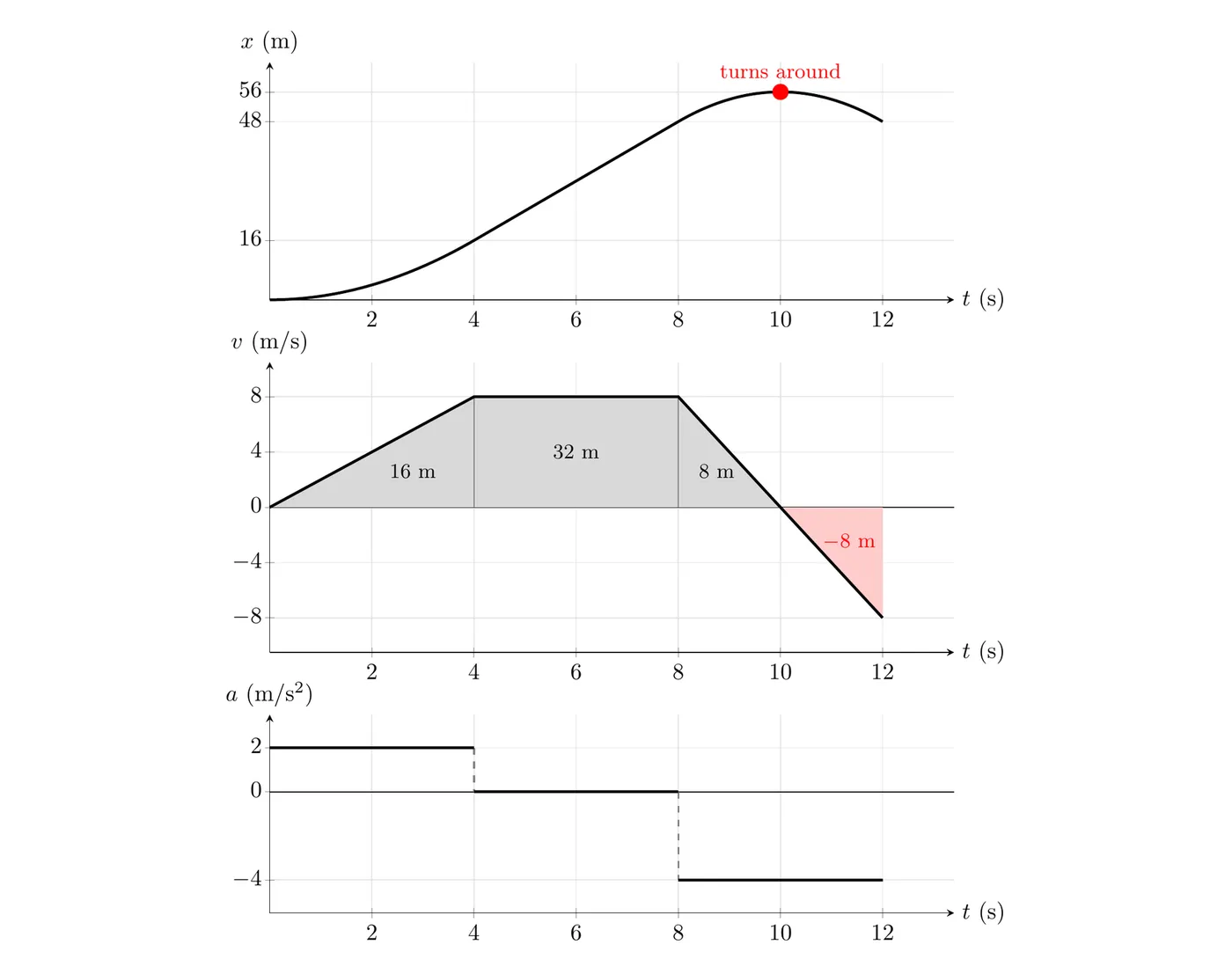
Find the acceleration at $t = 2.0$ s and at $t = 9.0$ s.

When is the cart farthest in the $+x$ direction, and where is it then?

Find the cart’s displacement and total distance from $t = 0$ to $t = 12$ s.

Part (a): Acceleration from Slopes

a(2.0) = \frac{8.0 - 0}{4.0 - 0} = 2.0 \text{ m/s}^2 \qquad a(9.0) = \frac{-8.0 - 8.0}{12 - 8.0} = -4.0 \text{ m/s}^2

Between 4 s and 8 s the graph is flat, so

a = 0

. Plotting these slopes gives the step-shaped acceleration graph.

Part (b): Farthest Point

The cart moves in the

+x

direction as long as

v > 0

. The velocity hits zero and changes sign at

t = 10

s, so that’s where it turns around. Its position there is the shaded area from 0 to 10 s:

x(10) = \frac{1}{2}(4.0)(8.0) + (4.0)(8.0) + \frac{1}{2}(2.0)(8.0) = 16 + 32 + 8.0 = 56 \text{ m}

Part (c): Displacement and Distance

From 10 s to 12 s the area is below the axis:

\frac{1}{2}(2.0)(-8.0) = -8.0

\Delta x = 56 + (-8.0) = 48 \text{ m} \qquad \text{distance} = 56 + 8.0 = 64 \text{ m}

The read: on the position graph, the slope matches the velocity at every instant. It curves upward while

v

increases (0 to 4 s), is a straight line while

v

is constant (4 to 8 s), levels off at the turnaround (

t = 10

s), and heads back down after that.

Special Case: Free Fall Near Earth’s Surface

Near Earth’s surface, objects feel a constant downward acceleration from gravity:

a_g = g \approx 10 \text{ m/s}^2

The direction is always downward, so it’s negative if you take up as positive.

Which value to use: - The AP Physics C exam uses

g = 10

m/s² whenever it needs a number, on both multiple choice and free response. - You won’t lose points for correctly using the more precise

g = 9.8

m/s² or

g = 9.81

m/s² instead (the equation sheet’s constants table lists 9.8 m/s²). - If a problem gives a specific value, always use that one.

Example: Ball Thrown Straight Up

Problem: you throw a ball straight up at 12 m/s. Take up as positive, so

a = -g = -10

m/s². How long does it take to reach the top, how high does it go, and how fast is it moving when it comes back to your hand?

At the top, the ball stops for an instant (

v = 0

0 = 12 + (-10)t \quad \Rightarrow \quad t = 1.2 \text{ s}

0 = (12)^2 + 2(-10)\Delta y \quad \Rightarrow \quad \Delta y = 7.2 \text{ m}

Back at your hand,

\Delta y = 0

0 = 12t + \frac{1}{2}(-10)t^2 = t(12 - 5t) \quad \Rightarrow \quad t = 2.4 \text{ s}

v = 12 + (-10)(2.4) = -12 \text{ m/s}

Answer: 1.2 s to the top, 7.2 m high, and it comes back at 12 m/s moving down (the negative sign). The trip up and the trip down take the same time.

At the top, $v = 0$ but $a$ is still $-10$ m/s². Gravity never switches off. If the acceleration were zero at the top, the ball would just stay there.

Example Problem: Chase Scenario

Problem: A cyclist travels at a constant 8 m/s in the positive x-direction. She passes a skateboarder who’s initially at rest. Just as she passes, the skateboarder starts accelerating at 0.8 m/s² in the positive x-direction.

How much time passes before the skateboarder catches up to the cyclist?

How far has the skateboarder traveled at that point?

How fast is the skateboarder going when they catch up?

Solution

Step 1: Write position equations for each object

Since both move in the positive x-direction, you can work with magnitudes.

The general displacement equation:

x = x_0 + v_0 t + \frac{1}{2}at^2

Cyclist: constant velocity, no acceleration. -

v_0 = 8

m/s -

a = 0

m/s²

x_{cyclist} = 8t

Skateboarder: starts from rest, constant acceleration. -

v_0 = 0

m/s -

a = 0.8

m/s²

x_{skateboarder} = \frac{1}{2}(0.8)t^2 = 0.4t^2

Part (a): Finding When They Meet

Set the positions equal:

8t = 0.4t^2

0.4t^2 - 8t = 0

Factor out

t

(don’t cancel it, or you’ll lose a solution):

t(0.4t - 8) = 0

That gives two solutions:

t = 0 \quad \text{(their initial meeting point)}

0.4t - 8 = 0

0.4t = 8

t = 20 \text{ seconds}

Answer: the skateboarder catches up after 20 seconds.

Part (b): Finding the Distance Traveled

They’re at the same position when they meet, so you can use either equation. The cyclist’s is simpler:

x = 8t = 8(20) = 160 \text{ m}

Check with the skateboarder’s equation:

x = 0.4t^2 = 0.4(20)^2 = 0.4(400) = 160 \text{ m} \checkmark

Answer: the skateboarder has traveled 160 meters.

Part (c): Finding the Skateboarder’s Final Velocity

Use the velocity equation for the skateboarder:

v = v_0 + at

v = 0 + (0.8)(20) = 16 \text{ m/s}

Answer: the skateboarder is going 16 m/s when they catch up.

A nice insight: the skateboarder is moving at twice the cyclist’s speed (16 m/s versus 8 m/s) when they meet. That makes sense, since the skateboarder had to catch up from behind.

Common Mistakes

Using kinematic equations with non-constant acceleration. The standard kinematic equations only work with constant acceleration. If the acceleration varies with time, you need calculus.

Canceling variables too early. In $0.4t^2 = 8t$ , don’t divide both sides by $t$ right away, because that throws out the $t = 0$ solution. Factor instead.

Confusing slope and area on graphs. Slope of the position graph is velocity. Slope of the velocity graph is acceleration. Area under the velocity graph is displacement. Area under the acceleration graph is change in velocity.

Forgetting that direction matters. Even in one dimension, define your positive and negative directions clearly. In free fall problems, decide whether up or down is positive and stick with it.

Using the wrong value for g. Check whether the problem wants $g = 9.8$ m/s² or $g = 10$ m/s². Also remember that $g$ is the magnitude, so add a negative sign if the direction is opposite your positive direction.

Misreading “catches up” problems. When one object catches another, they’re at the same position at that time, so set the position equations equal, not the velocity equations.

Back Next