

4.2 - Monopoly
Market Structure
A monopoly sits at the least competitive end of the spectrum:
- Single seller: the firm is the industry.
- Unique product: no close substitutes exist.
- High entry barriers: legal protections, control of key resources, or steep startup costs keep competitors out.
- Price seekers: with total market control, they set price rather than accept it.
Revenue, Demand, and Elasticity
Since the monopolist faces the entire market demand curve, price and quantity decisions are linked.
- To sell more, the monopolist has to lower price on all units.
- Since price drops for every unit, MR is always below price.
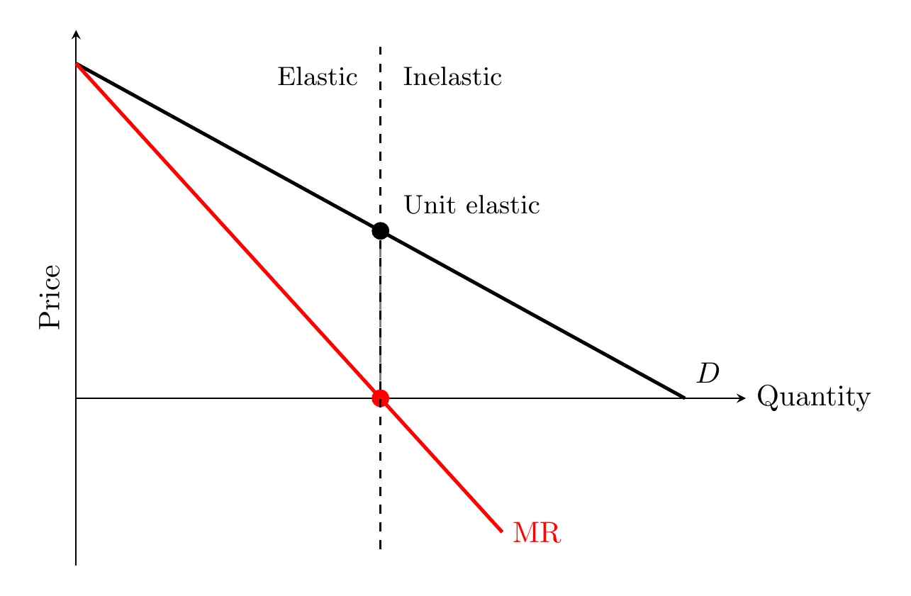
- Elasticity zones:
- MR positive → demand is elastic.
- MR zero → unit elastic, total revenue maximized.
- MR negative → demand is inelastic.
- Why it matters: a profit-maximizing monopoly always produces where demand is elastic. MC is always positive, so MR = MC can only happen where MR is positive, which is the elastic range. It will never pick a quantity on the inelastic part of demand.
Profit Maximization
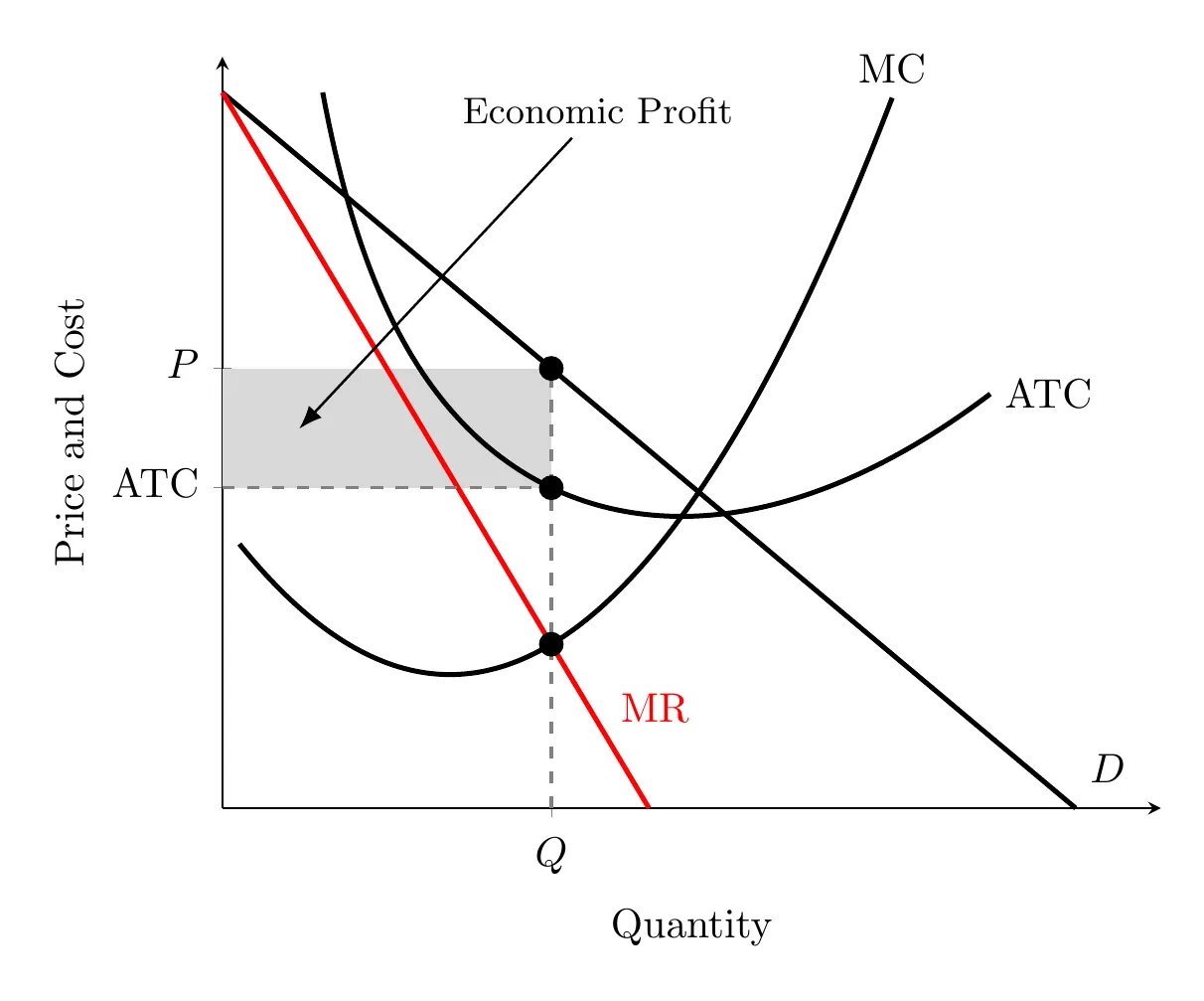
- Find quantity where MR = MC.
- Move up to the demand curve at that quantity to find the price.
- Compare price to ATC:
- Price above ATC → economic profit.
- Price equal to ATC → normal profit (breaking even).
- Price below ATC → economic loss.
Unlike competitive markets, a monopoly can sustain economic profit in the long run, since entry barriers keep competitors out.
Monopoly vs. Perfect Competition
Monopolies are generally less efficient, they charge more and produce less.
- Allocative inefficiency: society is best served where (the socially optimal quantity). A monopoly charges above MC, so it misses this.
- Deadweight loss: a triangle representing lost gains from trade that never happen because output is restricted.
- Productive inefficiency: the firm doesn’t produce at minimum ATC, often producing while ATC is still falling.
Calculating Surplus, Profit, and Deadweight Loss
AP questions often ask you to find these areas on a monopoly graph. Say a monopoly faces demand , so , and its MC and ATC are both a constant $4 (no fixed costs).
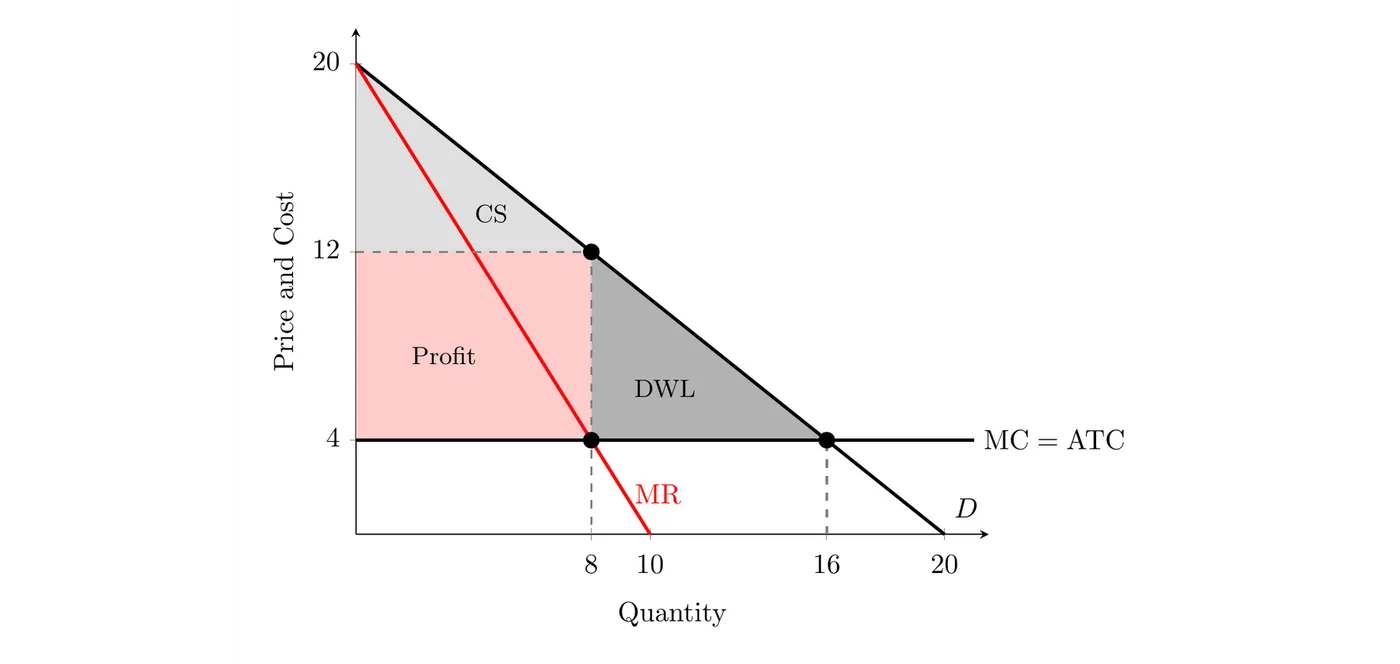
- Quantity and price: set MR = MC: 20 − 2Q = 4, so the monopoly makes 8 units. Go up to demand for the price: P = 20 − 8 = $12.
- Consumer surplus: the triangle under demand and above the price: ½ × 8 × ($20 − $12) = $32.
- Profit: the rectangle between price and ATC: ($12 − $4) × 8 = $64. Producer surplus is the area between price and MC, which is the same $64 here because there are no fixed costs. (With fixed costs, producer surplus is bigger than profit by the amount of the fixed cost.)
- Deadweight loss: the efficient quantity is where P = MC: 20 − Q = 4, so Q = 16. The DWL triangle sits between demand and MC from 8 to 16 units: ½ × (16 − 8) × ($12 − $4) = $32.
- Check: in a competitive market (P = MC = $4, Q = 16), consumer surplus would be ½ × 16 × ($20 − $4) = $128. The monopoly splits that same $128 into $32 of consumer surplus, $64 of profit, and $32 of deadweight loss that nobody gets.
That deadweight loss is why a monopoly’s price can’t be relied on to coordinate the market. Buyers would pay more than $4 for each unit from 8 to 16, and each one only costs $4 to make, but the monopoly won’t sell them. Selling more would mean cutting the price on all the units it already sells, so MR would fall below MC.
The Natural Monopoly
Sometimes a single provider actually is the more efficient outcome, thanks to extreme economies of scale.
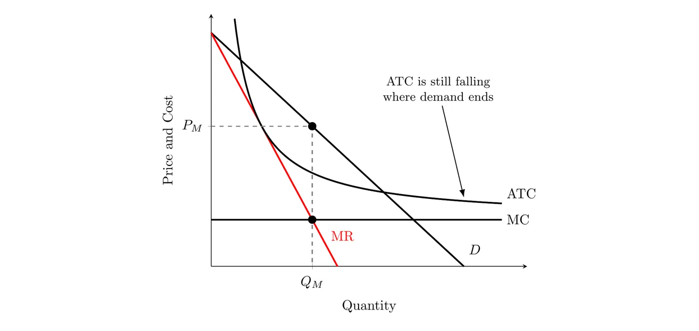
- Constantly declining costs: ATC keeps falling across all relevant levels of demand.
- Cost advantage: one big firm can serve the whole market cheaper per unit than several smaller firms could.
- Example: a citywide fiber-optic network. Laying the first cables is brutally expensive, but once it’s built, adding another house costs almost nothing. Five companies each digging up the same street to lay five sets of cable would just raise costs for everyone.
- Graph: ATC slopes down across the entire demand curve, even where demand hits the quantity axis. MC sits below ATC the whole way (when average cost is falling, marginal cost has to be below it). Left alone, a natural monopoly still acts like any monopoly: it makes the quantity where MR = MC and charges the price on the demand curve. (How governments regulate natural monopolies is in 6.4.)
Bottom line: a monopoly is a price seeker that uses total control to maximize profit at MR=MC, then charges whatever price the demand curve allows. High barriers let it sustain long-run profit, but society pays for it: less output, higher prices, deadweight loss, and no productive or allocative efficiency.