

6.4 - The Effects of Government Intervention in Different Market Structures
Why Intervene?
Ideally, intervention improves efficiency by fixing market failures. But there’s an important distinction:
- Corrective intervention: in markets with real failures (externalities, monopolies), good regulation reduces or eliminates deadweight loss.
- Distortive intervention: in perfectly competitive markets with no externalities, things like price controls or taxes actually create inefficiency and deadweight loss.
- What makes it work: a policy raises efficiency only if it fixes the incentive that caused the failure. A pollution tax works because it makes the polluter pay the external cost it was ignoring. A price ceiling works on a monopoly because the firm can no longer raise its price by cutting output. Get the size wrong (a tax bigger than the external cost, say) and the policy overcorrects, creating a new deadweight loss.
Regulating Monopoly Power
Monopolies and oligopolies naturally under-produce and overcharge ().
- Antitrust legislation promotes competition and blocks collusion, ideally raising output and lowering prices.
- Examples: the Sherman Antitrust Act (1890) bans monopolizing a market and agreements like price fixing, and the Clayton Act (1914) lets the government block mergers that would substantially reduce competition. In 1911 the Supreme Court used the Sherman Act to break up Standard Oil.
- Regulating natural monopolies (which have constantly falling ATC) usually means price ceilings:
- Fair-return price (): the firm breaks even, raising quantity and lowering price versus the unregulated outcome, leaving a smaller deadweight loss triangle.
- Allocatively efficient price (): wipes out deadweight loss entirely, but since ATC sits above price at this quantity, the firm takes a loss and needs a lump-sum subsidy to stay afloat.
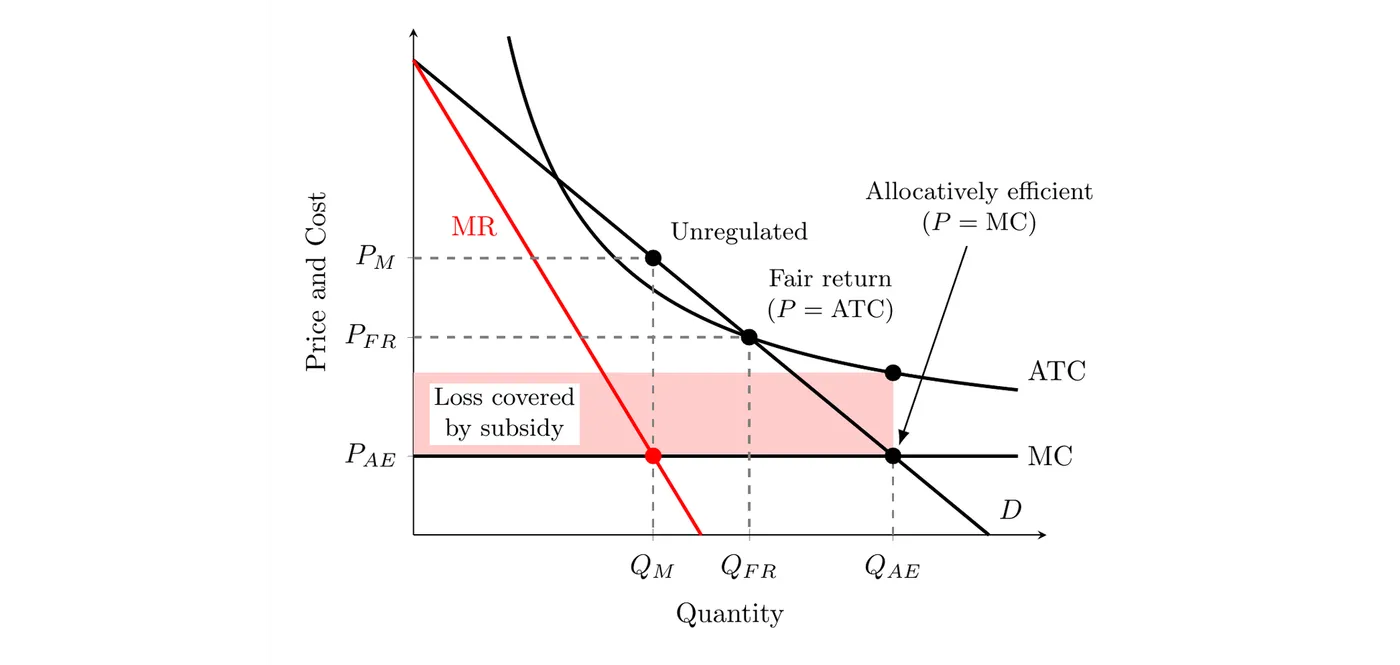
Reading the graph: unregulated, the natural monopoly produces (where MR = MC) and charges . A fair-return ceiling at , where demand crosses ATC, raises output to , and the firm breaks even. An allocatively efficient ceiling at , where demand crosses MC, raises output all the way to , but ATC is above price there. The shaded rectangle, , is the firm’s loss. A lump-sum subsidy that size keeps the firm in business without changing its marginal cost, so it keeps producing the efficient quantity.
Price Controls and Labor Markets
- Price floors (like minimum wage): set above equilibrium, they create a surplus. In labor markets, that means unemployment, worse if labor demand is elastic.
- Price ceilings: set below equilibrium, they create a shortage.
- The monopsony exception: unlike a competitive market, an effective minimum wage in a monopsony can actually raise both wages and employment while eliminating deadweight loss.
- This works best when the minimum wage is set where MRP crosses supply: the firm then hires the competitive quantity of workers. A minimum wage between the monopsony wage and that point still raises both wages and employment. Set it higher than that point, and employment starts falling again.
- Price ceilings on a monopoly: here a ceiling can actually raise output. Capped at the ceiling, the monopolist no longer has to cut its price to sell more, so each extra unit (up to what buyers want at that price) adds the full ceiling price to revenue. MR becomes flat at the ceiling.
- Ceiling below the monopoly price but above the point where MC crosses demand: the firm sells the quantity buyers demand at the ceiling, which is more than before, and deadweight loss shrinks.
- Ceiling right where MC crosses demand (): output hits the socially optimal quantity and deadweight loss disappears.
- Ceiling below that point: the firm only produces where MC equals the ceiling, so output falls and a shortage appears, just like in a competitive market.
- Monopolistic competition works the same way in the short run, since each firm also faces a downward-sloping demand curve. But in the long run these firms only break even (), so a ceiling below that price means losses, and some firms leave the market.
- Elasticity matters: the more elastic demand and supply are, the more quantities react to a price control, so the bigger the shortage from a ceiling or the surplus from a floor.
Taxes and Subsidies
- Per-unit taxes correct negative externalities by shifting supply to match MSC, reaching the socially optimal quantity and eliminating deadweight loss.
- Per-unit subsidies correct positive externalities by shifting demand to match MSB, reaching the optimal output.
- Lump-sum vs. per-unit:
- Per-unit taxes/subsidies shift both MC and ATC, changing the profit-maximizing price and quantity.
- Lump-sum taxes/subsidies only shift ATC, since MC doesn’t change, price and quantity stay the same.
What a per-unit tax or subsidy changes: the price buyers pay, the price sellers keep, the quantity, consumer and producer surplus, deadweight loss, and government revenue (for a tax) or cost (for a subsidy). How big each change is depends on the price elasticities of demand and supply.
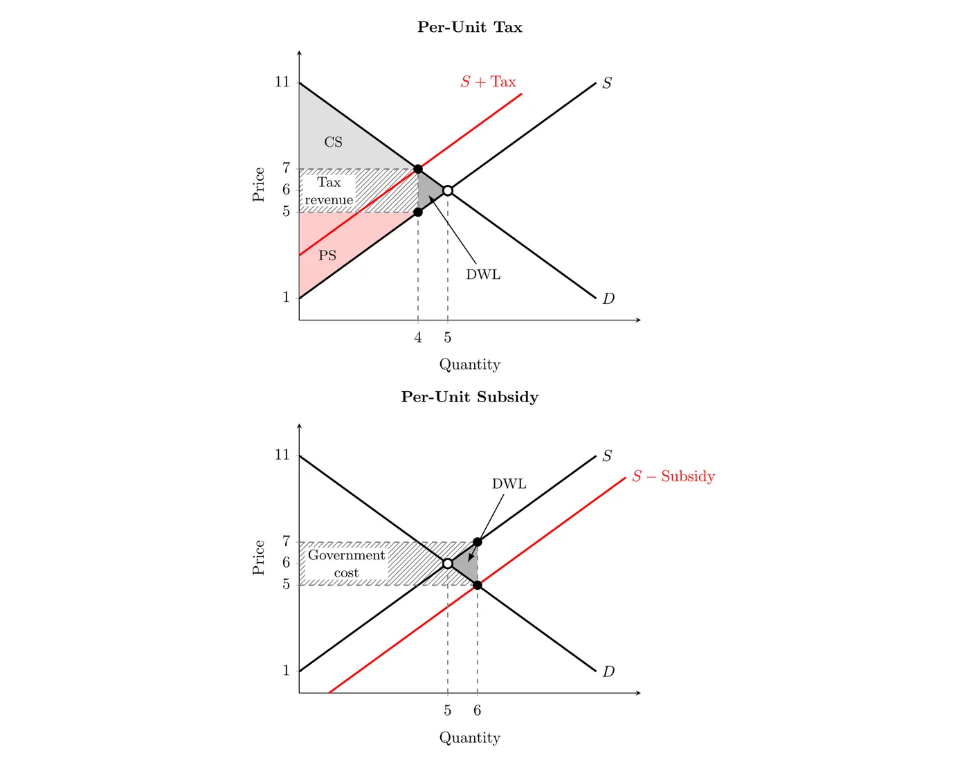
Example: demand is and supply is , so with no policy the market sells 5 units at $6. Consumer surplus is and producer surplus is , for a total of $25.
- $2 per-unit tax: supply shifts up by $2 to , so quantity falls to 4. Buyers pay $7 and sellers keep $5 (the $7 minus the $2 tax).
- CS = and PS = .
- Tax revenue = .
- DWL = . Check: , the original total.
- Buyers pay $1 more and sellers keep $1 less, so the burden splits evenly here because demand and supply are equally steep. In general, the less elastic side carries more of a tax (see 2.8).
- $2 per-unit subsidy: supply shifts down by $2 to , so quantity rises to 6. Buyers pay $5 and sellers receive $7 (the $5 plus the $2 subsidy).
- CS = and PS = , up $11 in total.
- Government cost = .
- DWL = . That’s the $12 the government spent minus the $11 buyers and sellers gained: the extra unit costs more to make than buyers value it.
- Elasticity: the more elastic demand and supply are, the more quantity changes, so the bigger the deadweight loss (and the less revenue a tax brings in).
Bottom line: government intervention cuts both ways. Applied to perfectly competitive markets, taxes and price controls usually create deadweight loss. But applied to actual market failures, monopolies, monopsonies, externalities, those same tools can fix the market, pushing output toward the socially optimal quantity and raising total welfare.