2.5 - Electric Potential

What Electric Potential Is

Electric potential (

V

) is the electric potential energy per unit charge at a point in space.

V = \frac{U_E}{q}

where: -

V

= electric potential (J/C = volt, V) -

U_E

= electric potential energy (J) -

q

= test charge (C)

The unit is the volt: 1 V = 1 joule/coulomb (J/C).

The distinction to keep straight: - Potential energy (

U_E

) is a property of a system of charges, measured in joules. - Potential (

V

) is a property of a point in space, measured in volts.

Potential is a scalar, so it has no direction, just a magnitude and a sign.

Electric Potential from Point Charges

A Single Point Charge

The potential at a distance

r

from a charge

Q

is:

V = \frac{1}{4\pi\epsilon_0}\frac{Q}{r} = k\frac{Q}{r}

where: -

V

= electric potential (V) -

k = 8.99 \times 10^9

N·m²/C² -

Q

= source charge (C), and you keep the sign -

r

= distance from the charge (m)

The reference point is

V = 0

r = \infty

. The sign follows the charge: - A positive charge (

Q > 0

) gives

V > 0

. - A negative charge (

Q < 0

) gives

V < 0

Multiple Point Charges (Superposition)

Potential adds as a scalar, so the total from several charges is just the algebraic sum, not a vector sum:

V_{total} = \frac{1}{4\pi\epsilon_0} \sum_i \frac{q_i}{r_i} = k\sum_i \frac{q_i}{r_i}

Written out:

V_{total} = k\left(\frac{q_1}{r_1} + \frac{q_2}{r_2} + \frac{q_3}{r_3} + ...\right)

where each

r_i

is the distance from charge

q_i

to the point you care about.

This is much easier than dealing with the electric field, since you just add numbers with their signs and never have to break anything into components.

On the AP exam you’ll only calculate the potential from four or fewer point charges (or more if the setup is very symmetric, like equal charges spaced evenly around a circle).

Electric Potential Difference

The potential difference (

\Delta V

) is the change in potential between two points.

\Delta V = V_f - V_i = \frac{\Delta U_E}{q}

Or:

\Delta V = \frac{W_{external}}{q}

where

W_{external}

is the work an external force does to move charge

q

from the starting point to the ending point at constant speed, so its kinetic energy doesn’t change.

Most people just call this voltage. Physically, it’s the work per unit charge needed to move a charge between two points.

How It Ties to Work and Energy

The work the electric field does on a charge

q

moving through a potential difference is:

W_{field} = -q\Delta V = q(V_i - V_f)

The change in kinetic energy is:

\Delta K = -\Delta U_E = -q\Delta V = q(V_i - V_f)

Sign-wise: - A positive charge moving from high

V

to low

V

loses PE and gains KE, so it speeds up. - A positive charge moving from low

V

to high

V

gains PE and loses KE, so it slows down.

Batteries

A battery creates a potential difference through chemical processes that separate charges: - The positive terminal is at high potential. - The negative terminal is at low potential. - It holds a constant

\Delta V

, which is its voltage rating, like a 9V battery.

Conductors and Potential

In electrostatic equilibrium, connected conductors sit at the same potential: - When conductors touch or are joined by a wire, charges redistribute. - Electrons flow until every surface reaches the same potential. - Once there’s no potential difference, there’s no field along the connection, so no more charge flows.

That gives a few properties: 1. The entire conductor is at the same potential, so it’s an equipotential. 2. The surface is an equipotential, with constant

V

everywhere on it. 3. The field inside is zero, so there’s no potential difference inside.

Two spheres joined by a wire: outside a charged sphere, the sphere acts like a point charge at its center (Topic 2.3), so its surface is at

V = k\frac{Q}{R}

. Connect two far-apart spheres with a thin wire, and charge flows until

k\frac{Q_1}{R_1} = k\frac{Q_2}{R_2}

. So the charge splits in proportion to the radii: the bigger sphere ends up with more charge, even though both end up at the same potential. Practice Problem 5 works through the numbers.

Relationship Between Electric Field and Potential

Getting the Field from a Potential Difference

The average electric field between two points separated by a distance

\Delta r

is:

|\vec{E}| = \frac{\Delta V}{\Delta r} = \frac{|V_f - V_i|}{\Delta r}

For a uniform field:

E = \frac{V}{d}

where

d

is the separation, which is common for parallel plates.

The field points from high potential to low potential, so it runs downhill.

The field points in the direction where the potential drops the fastest.

Key Relationships

Quantity	Field $\vec{E}$	Potential $V$
Type	Vector	Scalar
Point charge	$E = k\frac{Q}{r^2}$	$V = k\frac{Q}{r}$
Superposition	Vector sum	Algebraic sum
Direction	Away from + / Toward −	N/A (scalar)
Relation	$E = \left\|\frac{\Delta V}{\Delta r}\right\|$ , pointing toward lower $V$	$\Delta V = -Ed$ for a move of $d$ along a uniform $\vec{E}$

Equipotential Lines (Isolines)

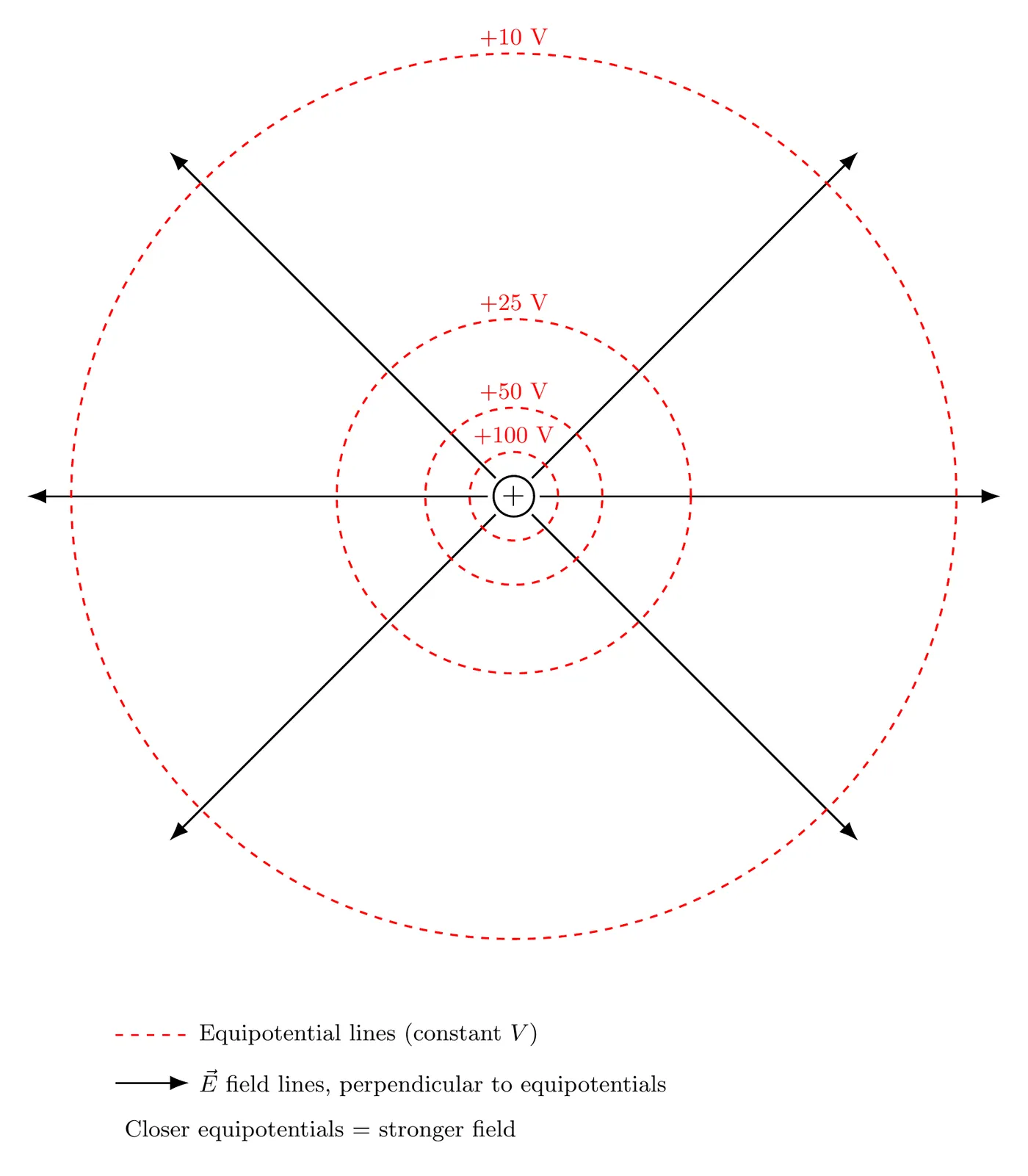
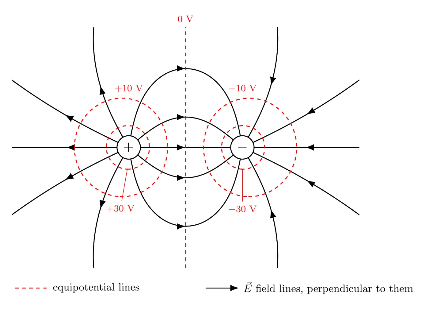
An equipotential line, or isoline, is a line or surface where the potential is constant. Its properties: 1. It’s perpendicular to the electric field lines everywhere. 2. It takes no work to move a charge along it, since there’s no

\Delta V

. 3. There’s no component of

\vec{E}

along it, because the field is perpendicular. 4. Closer spacing means a stronger field, since the potential changes more steeply. 5. Equipotentials never cross each other.

Going back and forth between the two maps: - From a field vector map to an isoline map: draw lines that cross every field vector at a right angle. If each line is the same

\Delta V

from the next, they bunch up where the vectors are longest. - From an isoline map to a field vector map: draw arrows perpendicular to the isolines, pointing toward lower

V

. Make them longer where the isolines are closer together. - Predicting motion: a positive charge feels a force along

\vec{E}

, toward lower potential. A negative charge feels a force the other way, toward higher potential.

Parallel Plates (Uniform Field)

Between uniformly charged parallel plates: - The equipotential lines run parallel to the plates. - They’re equally spaced, since the field is uniform. - The field is perpendicular to the plates.

E = \frac{V}{d}

where

V

is the potential difference between the plates and

d

is the separation.

Practice Problem 1: Potential from a Point Charge

Problem: Find the electric potential 0.50 m from a point charge

Q = +6.0 \times 10^{-9}

Solution:

V = k\frac{Q}{r} = (8.99 \times 10^9)\frac{6.0 \times 10^{-9}}{0.50}

V = 108 \text{ V}

Answer: 108 V, positive because the source charge is positive.

Practice Problem 2: Superposition of Potentials

Problem: Two charges are fixed in place:

q_1 = +4.0

μC at the origin and

q_2 = -2.0

μC at

x = 0.30

m. Find the potential at

x = 0.10

Solution:

Distance from

q_1

r_1 = 0.10

m. Distance from

q_2

r_2 = 0.30 - 0.10 = 0.20

Potential from

q_1

V_1 = k\frac{q_1}{r_1} = (8.99 \times 10^9)\frac{4.0 \times 10^{-6}}{0.10} = 3.60 \times 10^5 \text{ V}

Potential from

q_2

V_2 = k\frac{q_2}{r_2} = (8.99 \times 10^9)\frac{-2.0 \times 10^{-6}}{0.20} = -8.99 \times 10^4 \text{ V}

Total (algebraic sum):

V_{total} = V_1 + V_2 = 3.60 \times 10^5 - 8.99 \times 10^4 = 2.70 \times 10^5 \text{ V}

Answer:

2.7 \times 10^5

Practice Problem 3: Potential Difference and Energy

Problem: A proton is accelerated from rest through a potential difference of 1000 V. What is its final kinetic energy, in both eV and joules?

Solution:

The change in kinetic energy equals the negative change in potential energy:

\Delta K = -\Delta U_E = -q\Delta V

For a proton,

q = +e

\Delta K = -e(V_f - V_i) = -e(0 - 1000 \text{ V}) = e(1000 \text{ V})

In eV:

\Delta K = 1000 \text{ eV} = 1.0 \text{ keV}

In joules:

\Delta K = 1000 \times (1.60 \times 10^{-19}) = 1.60 \times 10^{-16} \text{ J}

Answer: 1000 eV, or

1.6 \times 10^{-16}

Quick note: when a charge

q

moves through a potential difference

\Delta V

, it gains or loses energy

q|\Delta V|

. For elementary charges, the electronvolt (eV) is a handy unit.

Practice Problem 4: Field from Potential

Problem: The potential difference between two parallel plates 2.0 cm apart is 500 V. What is the magnitude of the field between them?

Solution:

E = \frac{\Delta V}{d} = \frac{500}{0.020} = 2.5 \times 10^4 \text{ N/C}

Answer:

2.5 \times 10^4

N/C, pointing from the positive plate to the negative plate.

Practice Problem 5: Conductors Connected by a Wire

Problem: Metal sphere A (radius 10 cm) has a charge of

+6.0

nC. Metal sphere B (radius 5.0 cm) is neutral. The spheres are far apart, and they get connected by a long, thin wire. Find: (a) the charge on each sphere afterward (b) the potential of each sphere afterward

Solution:

Charges:

Charge is conserved (the thin wire holds almost none), so

Q_A + Q_B = 6.0

nC. The spheres end up at the same potential:

k\frac{Q_A}{R_A} = k\frac{Q_B}{R_B} \quad\Rightarrow\quad Q_A = \frac{R_A}{R_B}Q_B = \frac{10}{5.0}Q_B = 2Q_B

2Q_B + Q_B = 6.0 \text{ nC} \quad\Rightarrow\quad Q_B = 2.0 \text{ nC}, \quad Q_A = 4.0 \text{ nC}

Potential:

V_A = k\frac{Q_A}{R_A} = (8.99 \times 10^9)\frac{4.0 \times 10^{-9}}{0.10} = 3.6 \times 10^2 \text{ V}

V_B = k\frac{Q_B}{R_B} = (8.99 \times 10^9)\frac{2.0 \times 10^{-9}}{0.050} = 3.6 \times 10^2 \text{ V}

Answer: (a)

Q_A = +4.0

nC and

Q_B = +2.0

nC, (b) both are at about 360 V.

What actually moved? Before the wire, A was at

(8.99 \times 10^9)(6.0 \times 10^{-9})/0.10 \approx 540

V and B was at 0 V. Electrons flowed from B to A (toward higher potential) until both were at 360 V. B lost 2.0 nC worth of electrons, which is why it ended up positive.

Notice the small sphere has less charge but the stronger field at its surface:

E = kQ/R^2

gives about

3.6 \times 10^3

N/C for A and

7.2 \times 10^3

N/C for B. That’s the same reason charge piles up at sharp points (Topic 2.3).

Practice Problem 6: Reading an Equipotential Map

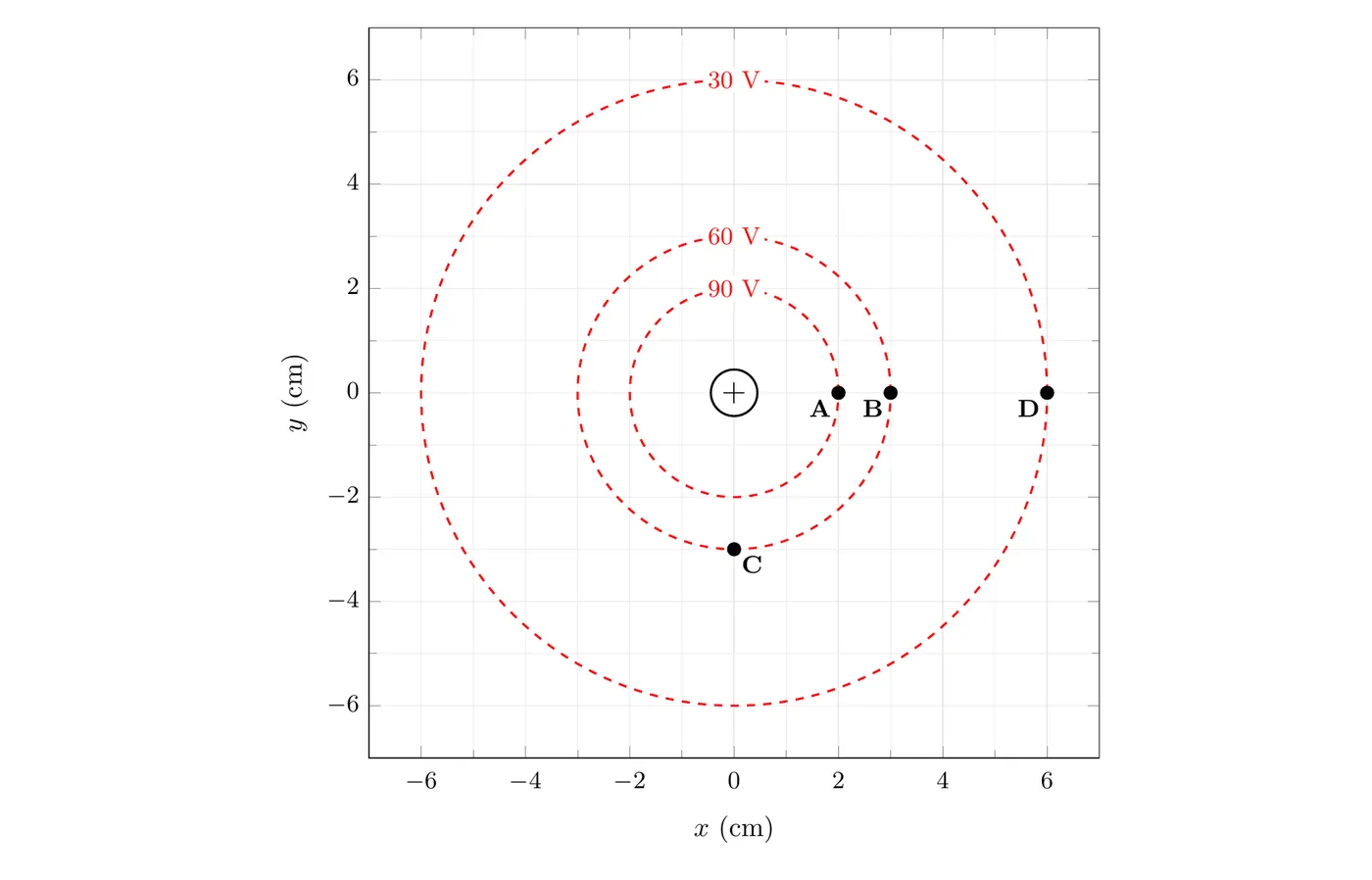
Problem: The map shows equipotential lines (red, dashed) around a small charged sphere at the origin. Points A, B, C, and D sit on the lines. (a) What is the sign of the sphere’s charge, and which way does the field point at B? (b) Estimate the average field strength between A and B, and between B and D. (c) How much work does the field do on a

+5.0

nC charge that moves from A to D? (d) How much work does the field do on that charge if it moves from B to C? (e) An electron is released from rest at B. Which way does it start to move?

Solution:

The potential drops as you move away from the sphere, and the field points toward lower potential, so it points outward. Field lines point away from positive charges, so the sphere is positive. At B, $\vec{E}$ points in the +x direction, perpendicular to the 60 V line.

Use $E = \left|\frac{\Delta V}{\Delta r}\right|$ with distances read off the grid:

E_{AB} = \frac{|60 - 90| \text{ V}}{0.010 \text{ m}} = 3.0 \times 10^3 \text{ V/m}

E_{BD} = \frac{|30 - 60| \text{ V}}{0.030 \text{ m}} = 1.0 \times 10^3 \text{ V/m}

It’s the same 30 V step each time, but the lines are 3 times closer together between A and B, so the field there is 3 times stronger.

The field’s work is $W = -q\Delta V$ :

W_{A \to D} = -(5.0 \times 10^{-9})(30 - 90) = +3.0 \times 10^{-7} \text{ J}

B and C are both on the 60 V line, so $\Delta V = 0$ and $W = 0$ . That’s true for any path from B to C, not just along the line, because the work only depends on the starting and ending potentials.

An electron is pushed opposite to $\vec{E}$ , toward higher potential. So it starts moving in the $-x$ direction, toward the sphere.

Answer: (a) positive, and

\vec{E}

points in the +x direction at B, (b) about

3.0 \times 10^3

V/m and

1.0 \times 10^3

V/m, (c)

+3.0 \times 10^{-7}

J, (d) 0, (e) toward the sphere (

-x

These are averages. The field near a point charge changes smoothly with distance, so

\Delta V/\Delta r

gives the average over the gap, not the exact value at one point.

Common Mistakes

Confusing potential and potential energy. Potential energy ( $U_E$ ) depends on the arrangement of charges and is measured in joules. Potential ( $V$ ) is a property of a point in space, measured in volts.

Doing vector addition instead of scalar. Potential is a scalar, so just add with signs. No components needed.

Forgetting signs. Keep the signs of the charges. A positive charge gives a positive potential and a negative charge gives a negative potential.

Using the wrong reference point. $V = 0$ is at infinity, like PE, not at the charge’s location.

Mixing up high and low potential. A positive charge naturally moves from high to low $V$ and gains KE, and the field also points from high to low $V$ , so downhill.

Thinking equipotentials and field lines are parallel. They’re perpendicular, not parallel.

Getting the direction of $\Delta V$ wrong. $\Delta V = V_f - V_i$ . Moving from 10 V to 5 V gives $\Delta V = -5$ V, a decrease.

Using the wrong distance. For potential at a point, $r$ is the distance from the source charge to that point, not the distance between two charges.

Forgetting the uniform field shortcut. Between parallel plates, $E = V/d$ is simpler than the general formulas.

Thinking work is zero because PE decreased. If $\Delta U_E < 0$ , the field did positive work. If you want the external work against the field, it has the opposite sign.

Back Next