

6.2 - Electromagnetic Induction
Faraday’s Law of Induction
Faraday’s Law connects a changing magnetic flux to the electromotive force (EMF) it induces in a circuit.
The Math
Written out more fully:
where:
- = induced EMF (V, volts).
- = magnetic flux (Wb, webers).
- = magnetic field strength (T).
- = area of the loop (m²).
- = angle between and .
What it means: a changing magnetic flux through a loop induces a voltage in that loop.
The key insight: it’s the rate of change that counts. A static magnetic field, however strong, induces nothing.
Three Ways to Change the Flux
Magnetic flux can change in three ways:
- Change the field strength (so varies with time).
- Move a magnet toward or away from the loop.
- Crank the current in a nearby electromagnet up or down.
- Change the area (so varies with time).
- Stretch or squeeze the loop.
- Slide a conducting bar to change the enclosed area.
- Change the angle (so varies with time).
- Spin a loop in a magnetic field.
- Tilt its orientation relative to the field.
Any of the three induces an EMF, because all three change .
Coils with N Turns
Real coils have many turns. The same flux passes through each turn, so each turn gets the same EMF. The turns are connected one after another (in series), so their EMFs add up:
This is the form on the AP equation sheet, where is the flux through one turn. It works for a long solenoid or any tightly wound coil.
Example: A flat coil has 200 turns, each with radius 0.040 m, and a total resistance of 4.0 Ω (its two ends are connected). A uniform field along the coil’s axis drops steadily from 0.60 T to 0.20 T in 0.25 s. Find the size of the induced EMF and the current.
With just one turn, the EMF would be only 8.0 mV. The 200 turns multiply it by 200.
Constant Area or Constant Field
Two special cases of show up all the time.
The area stays the same and the field changes. The EMF is the area times how fast the part of the field perpendicular to the surface changes:
The coil example above and the Example Problem later on this page are both this case.
The field stays the same and the area changes. The EMF is the field times how fast the area perpendicular to the field changes:
Example: A circular loop of stretchy conducting material sits in a uniform 0.50 T field perpendicular to its plane. Its radius grows at 0.050 m/s. Find the EMF at the moment the radius is 0.20 m.
The area is , so by the chain rule:
Since depends on , the EMF keeps growing as the loop gets bigger, even though the radius grows at a steady rate.
A rotating coil counts too. The area perpendicular to the field is . Spin a coil of turns at a steady angular speed , so :
The EMF is biggest when , which is when the coil’s plane lines up with the field. The flux is zero at that moment, but it’s changing fastest. That’s how a generator works. For example, a 50-turn coil with area 0.020 m² spinning at 120 rad/s in a 0.30 T field has a peak EMF of V.
Lenz’s Law: What That Negative Sign Is Doing
The negative sign in Faraday’s Law is Lenz’s Law, and it’s what tells you the direction of the induced current.
The Statement
The induced current flows in whatever direction opposes the flux change that created it.
One way to think about it: nature pushes back against change. The induced current makes its own magnetic field that tries to hold things the way they were.
How to Apply It
Step 1: figure out whether the flux through the loop is going up or going down.
Step 2: figure out which way the external field points through the loop.
Step 3: apply the rule:
- Flux increasing: the induced field fights it, pointing opposite the external field.
- Flux decreasing: the induced field props it up, pointing the same way as the external field.
Step 4: use the right-hand rule to find the current direction that produces that induced field.
Getting the Direction from the Sign
The right-hand rule ties together the current, the EMF, and the flux. Here’s a second way to get the direction, using the sign in Faraday’s Law:
- Pick a positive direction around the loop (say counterclockwise). Curl your right-hand fingers that way. Your thumb gives the direction of .
- Find using that . Flux along your thumb is positive.
- Compute . If comes out positive, the induced current flows the way you picked. If it’s negative, it flows the other way.
The two methods always agree. Lenz’s Law is the quick picture, and the sign is what the math gives you.
Visual Examples: Magnet Moving Through a Loop
Let’s walk through what happens with a bar magnet and a wire loop.
Scenario A: Nothing Moving (No Induced EMF)
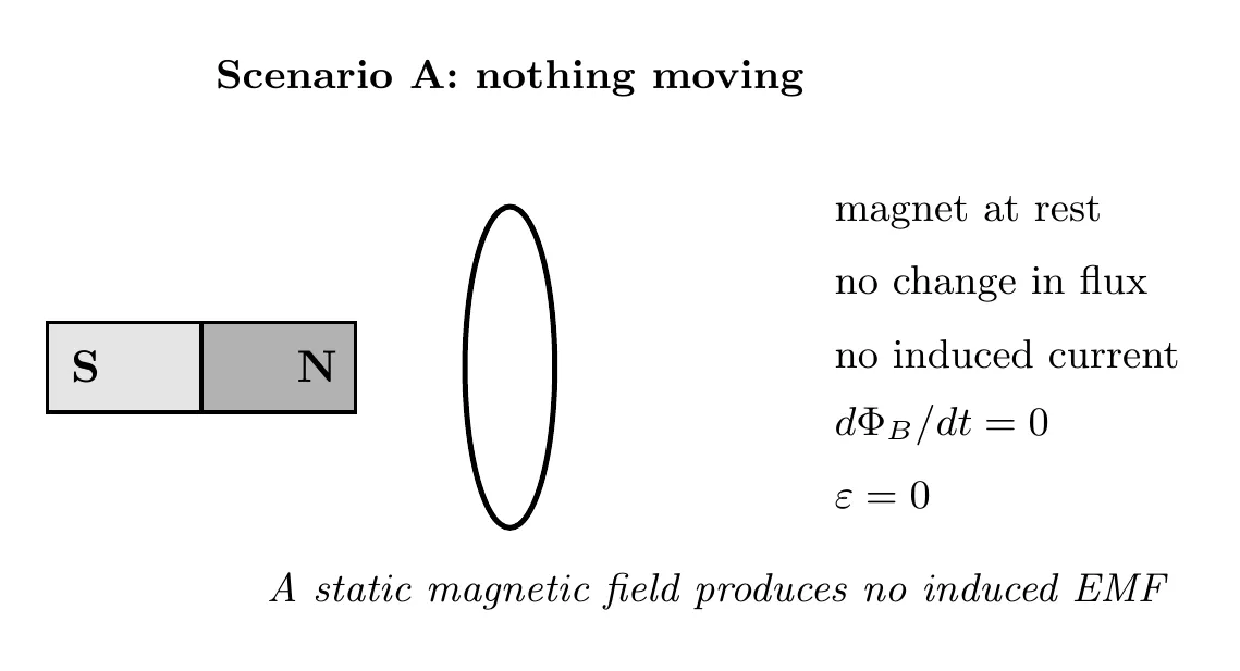
Why no current? The flux through the loop isn’t changing, so , which means .
Scenario B: North Pole Coming In (Flux Increasing)
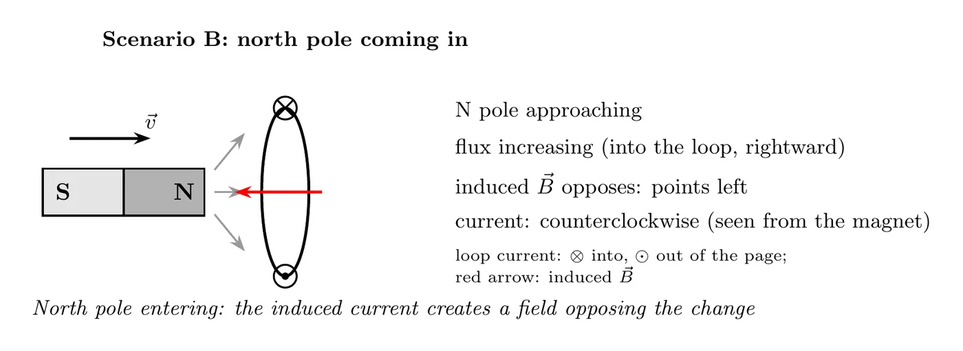
Breaking it down:
- The external field through the loop is increasing, since more field lines are coming in.
- That external field points into the loop, toward the right.
- The induced field has to fight the increase, so it points out of the loop, toward the left.
- Current direction: counterclockwise. Use the right-hand rule, curling your fingers with the current so your thumb points along the induced field.
Scenario C: North Pole Leaving (Flux Decreasing)
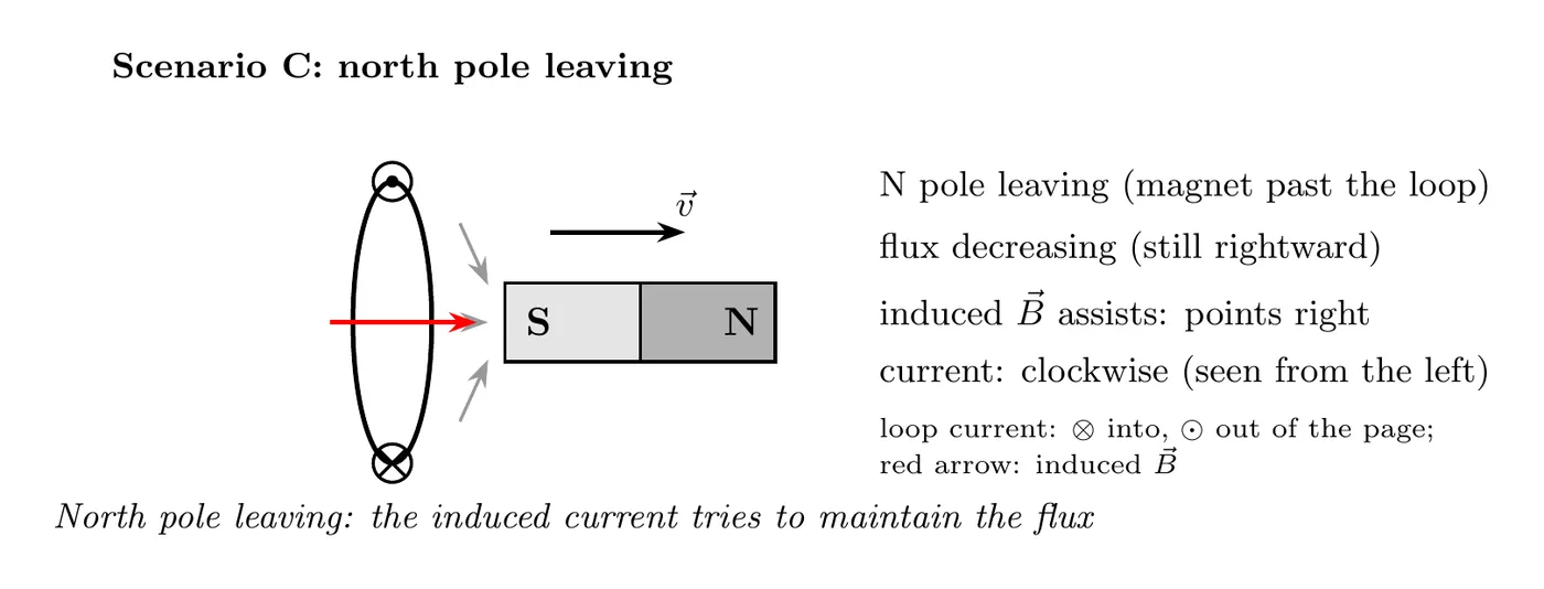
Breaking it down:
- The external field through the loop is decreasing, since there are fewer field lines.
- It still points into the loop, toward the right, but it’s fading.
- The induced field has to prop it up to fight the decrease, so it points into the loop too, toward the right.
- Current direction: clockwise. Curl clockwise and your thumb points right.
Scenario D: South Pole Coming In (Flux Increasing the Other Way)
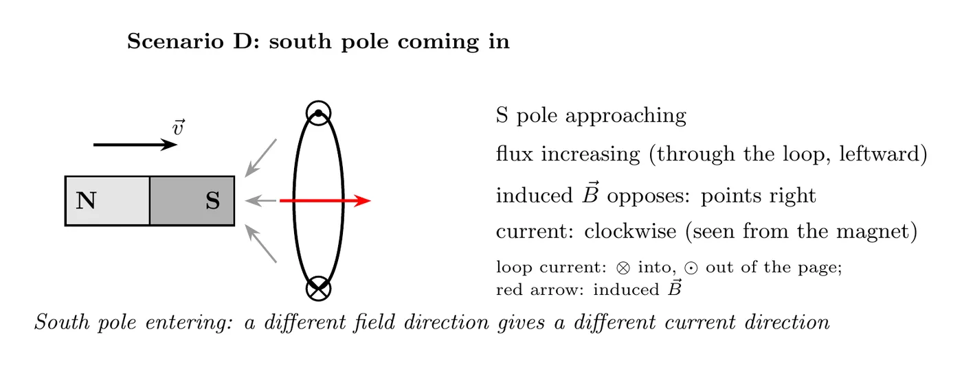
Breaking it down:
- The external field through the loop is increasing.
- It points from right to left, toward the S pole.
- The induced field has to fight the increase, so it points from left to right, the opposite way.
- Current direction: clockwise.
Scenario E: South Pole Leaving (Flux Decreasing)
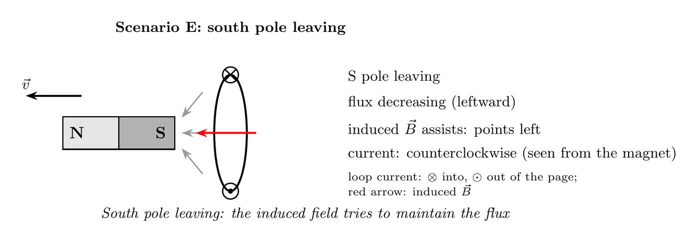
Breaking it down:
- The external field through the loop is decreasing.
- It points from right to left.
- The induced field has to prop it up to fight the decrease, so it also points from right to left.
- Current direction: counterclockwise.
Summary Table: Applying Lenz’s Law
Scenario | Flux Change | External Field Direction | Induced Field Direction | Current Direction |
N entering | Increasing | Into loop (right) | Fights it: out of loop (left) | Counterclockwise |
N leaving | Decreasing | Into loop (right) | Props it up: into loop (right) | Clockwise |
S entering | Increasing | Out of loop (left) | Fights it: into loop (right) | Clockwise |
S leaving | Decreasing | Out of loop (left) | Props it up: out of loop (left) | Counterclockwise |
The pattern to spot:
- Magnet coming in (either pole): the induced field opposes the external field.
- Magnet leaving (either pole): the induced field reinforces the external field.
Example Problem: Lenz’s Law Near a Wire
Problem: Use the wire and loop from the flux example in topic 6.1: the loop’s long sides are 0.30 m long, at 0.050 m and 0.15 m from the wire. Now the current in the wire is increasing at 50 A/s, and the loop has a resistance of 0.010 Ω. (a) Which way does the induced current flow? (b) How big is the induced EMF? (c) Which way is the net magnetic force on the loop?
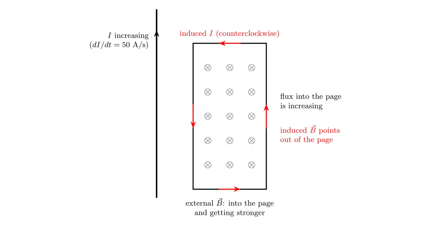
(a) Direction
Breaking it down:
- To the right of the wire, the wire’s field points into the page.
- The current is increasing, so that field gets stronger and the flux into the page is increasing.
- The induced current has to fight the increase, so its own field inside the loop points out of the page.
- Curl your right-hand fingers so your thumb points out of the page: the current runs counterclockwise.
(b) Size of the EMF
From topic 6.1, . Only changes, so:
That drives a current of A (0.33 mA) around the loop.
(c) Force on the loop
Breaking it down:
- Left side (near the wire): the induced current runs down, opposite to the wire’s current. Opposite currents repel, so this side is pushed away from the wire.
- Right side (far side): the current runs up, the same way as the wire’s current, so this side is pulled toward the wire. But the field is 3 times weaker out there, so this force is 3 times smaller.
- Top and bottom: equal and opposite forces that cancel.
- Net force: away from the wire.
What it tells you: the loop gets pushed toward weaker field, where less flux would pass through it. That’s Lenz’s Law again: the force opposes the change that caused the current. Topic 6.3 covers these forces in more detail.
Faraday’s Law as Maxwell’s Third Equation
Faraday’s Law is the third of Maxwell’s four equations:
What it says: a changing magnetic flux creates a circulating electric field.
This is a new kind of electric field. It isn’t made by charges. It’s made by a changing magnetic field, and it shows up whether or not there’s a wire there. A wire loop just gives the field some charges to push around, and that’s the induced current. A few things make it different from the electric fields in Units 1 to 3:
- Its field lines are closed loops. They don’t start or end on charges.
- Going once around a closed path, it does nonzero work on a charge. Per coulomb, that work is . So it’s not conservative, and you can’t describe it with an electric potential.
- The EMF of a loop is this integral. The equation sheet puts both forms together: .
Example: The Induced Electric Field Around a Changing Field
Problem: Inside a long solenoid of radius m, the uniform field points into the page and increases at 0.080 T/s. Outside the solenoid, . Find the induced electric field (a) 0.050 m from the axis and (b) 0.30 m from the axis.
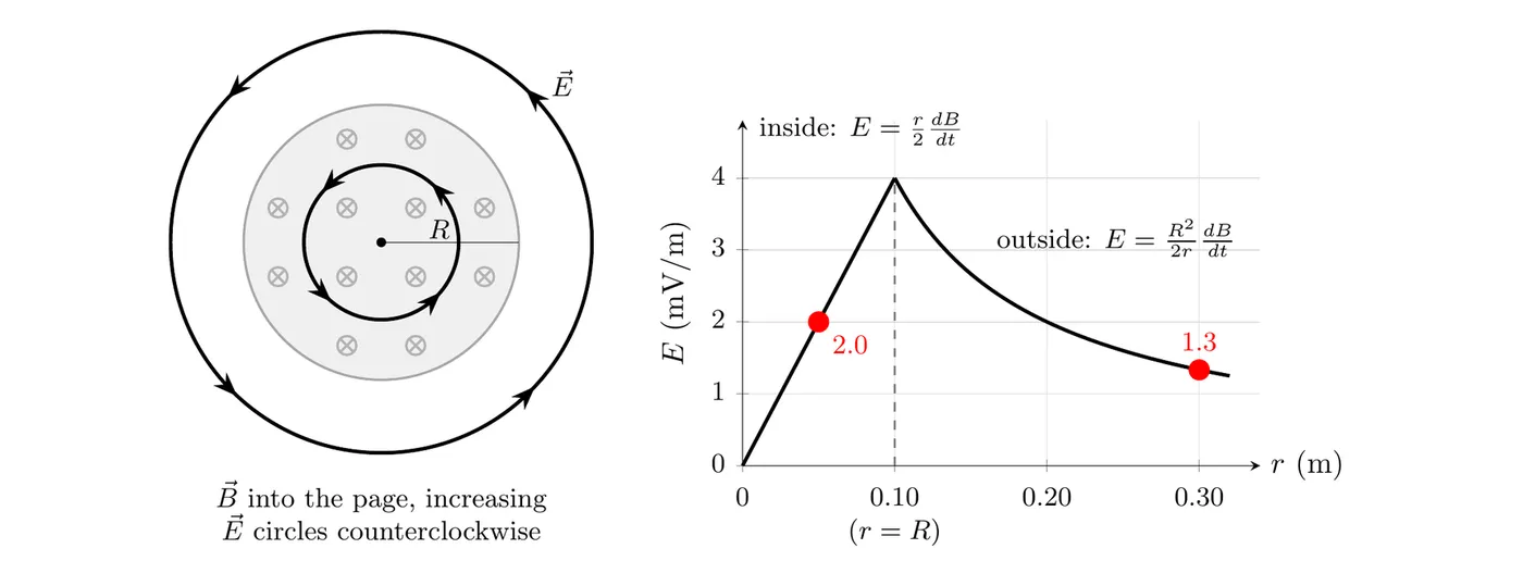
Setup: by symmetry, circles around the axis and has the same size everywhere on a circle of radius . Use that circle as the path, so . The field into the page is increasing, so by Lenz’s Law circles counterclockwise.
(a) Inside the solenoid
The circle encloses flux :
(b) Outside the solenoid
The circle encloses all of the solenoid’s flux, , and no more:
What it tells you: there’s an electric field at 0.30 m even though there. Inside, grows in proportion to . Outside, it falls off as . It peaks at the solenoid’s edge, .
The complete set of Maxwell’s equations:
- Gauss’s Law (electricity):
- Gauss’s Law (magnetism):
- Faraday’s Law:
- Ampère-Maxwell Law:
Look at the symmetry between equations 3 and 4:
- Changing magnetic flux makes an electric field (Faraday).
- Changing electric flux makes a magnetic field (Maxwell’s addition to Ampère).
- That symmetry is what makes electromagnetic waves possible.
Maxwell’s equations can be combined to show that and obey wave equations. The waves they describe are electromagnetic waves, and in empty space they all travel at the same speed:
Check it with the constants from the table of information:
That’s the speed of light, which is how Maxwell figured out that light is an electromagnetic wave. The AP course doesn’t ask you to derive this, but you should know the result and that it comes from Maxwell’s equations.
Example Problem: Induced Current from a Time-Varying Field
Problem:
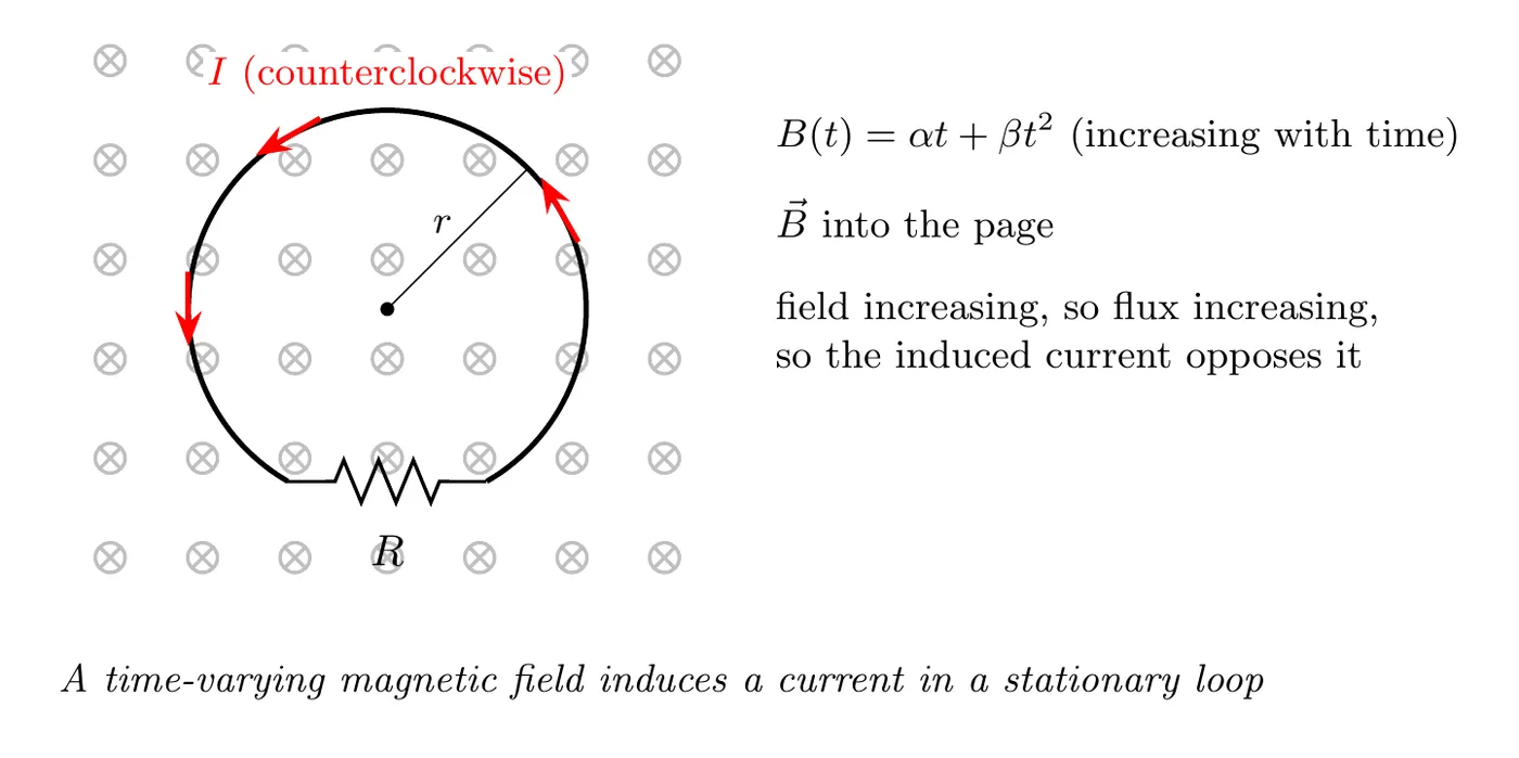
A circular loop of wire sits at rest with radius and resistance . It’s in a magnetic field pointing into the page, and the field’s magnitude changes with time as:
where and are positive constants with units of T/s and T/s² respectively.
Derive an expression for the current in the loop as a function of time.
Solution
Step 1: link current to the induced EMF with Ohm’s Law
Solve for current:
Step 2: get the induced EMF from Faraday’s Law
We’ll just take the magnitude here and sort out the direction separately:
Step 3: write down the magnetic flux
The field is perpendicular to the loop, so and:
And for a circular loop:
Step 4: plug in the time-varying field
Step 5: take the time derivative
The is constant, since the loop isn’t changing size:
Step 6: that’s the induced EMF
Step 7: get the current
Direction (from Lenz’s Law):
- The field into the page is increasing, since and .
- So the induced current has to make a field out of the page to fight the increase.
- By the right-hand rule, the current runs counterclockwise when viewed from above.
What it tells you:
- The current climbs linearly with time, thanks to the term.
- There’s also a constant piece from the term.
- A bigger loop (bigger ) means more flux change, which means more current.
- Bigger resistance () means less current, exactly as Ohm’s Law would have it.
Key Concepts Summary
Faraday’s Law
Three ways to change the flux:
1. Change (the field strength).
2. Change (the loop area).
3. Change (the orientation).
Lenz’s Law (the negative sign)
The induced current opposes whatever change caused it.
The rules:
- Flux increasing: the induced field points opposite the external field.
- Flux decreasing: the induced field points the same way as the external field.
Right-Hand Rule for Induced Current
- Curl your fingers the way the current flows.
- Your thumb points along the induced magnetic field.
Common Mistakes
- Forgetting that only CHANGING flux induces an EMF. A constant magnetic field, no matter how strong, gives you zero induced EMF. People think “strong field means big EMF,” but it’s the rate of change () that matters.
- Getting Lenz’s Law backwards. The induced field opposes the change, not the field itself. If the flux is going up, the induced field fights the increase and points the other way. If the flux is going down, the induced field fights the decrease and points the same way to try to hold it steady.
- Mixing up “into the page” and “out of the page.” Use ⊗ for into the page (the tail of the arrow) and ⊙ for out of the page (the point of the arrow). When you’re applying Lenz’s Law, be really careful about which way the external field points and which way the induced field has to point.
- Using the right-hand rule wrong. To find the current direction from the induced field, curl your fingers the way the current flows and your thumb gives the field that current makes. Don’t reach for the force rule, that’s for a different situation.
- Mixing up absolute value and signed value. Faraday’s Law has that negative sign for Lenz’s Law. When you’re calculating the magnitude of the current or EMF, you usually work with and figure out the direction separately. Don’t drag the negative sign through every calculation when you only want a magnitude.