5.1 - Rotational Kinematics

Introduction to Rotational Quantities

In Units 5 and 6, we take everything we know about linear (translational) motion and extend it to rotational (angular) motion. The core idea is simple: take the linear quantities and stick “angular” or “rotational” in front of them.

The math stays similar. You just use different symbols and interpret them in terms of rotation instead of straight-line motion.

Rigid Systems vs. Objects

Up to now, we’ve mostly modeled things as an object: a single point with mass and no size. That model can’t describe spinning. For rotation we use a rigid system: a system that holds its shape (it doesn’t stretch, bend, or squish), but whose points move in different directions while it rotates. On a turning wheel, the top moves forward, the bottom moves backward, and the axle barely moves at all. A rigid system can’t be modeled as an object, because a single point can’t tell one side of the wheel from the other or say where a force acts, and that’s exactly what decides whether something starts to spin (torque, in 5.3).

When you can ignore the rotation: if the motion you care about is well described by the motion of the system’s center of mass, you can still treat the system as a single object. For example, Earth spins once a day, but that spin is negligible when you study Earth’s yearly trip around the center of mass of the Earth-Sun system, so Earth is treated as an object there. The same thing can be an object in one problem and a rigid system in the next: a thrown football is an object when you find how far it travels, and a rigid system when you ask how fast it spins.

Angular Displacement

Angular displacement (

\theta

) is the angle, in radians, through which a point on a rigid system rotates about a specific axis.

As an equation, the angular displacement is the final angular position minus the initial one:

\Delta\theta = \theta - \theta_0

Units: radians (rad).

Sign convention: - Counterclockwise rotation is positive (+). - Clockwise rotation is negative (−).

Which direction counts as positive is a choice. One direction (clockwise or counterclockwise) is picked as mathematically positive, and the other becomes negative. Counterclockwise positive is the usual choice, but if everything in a problem turns clockwise, you can make clockwise positive instead, as long as every angular quantity in that problem uses the same choice. Clockwise and counterclockwise also depend on where you look from, so state the viewpoint (for example, looking down on a turntable from above).

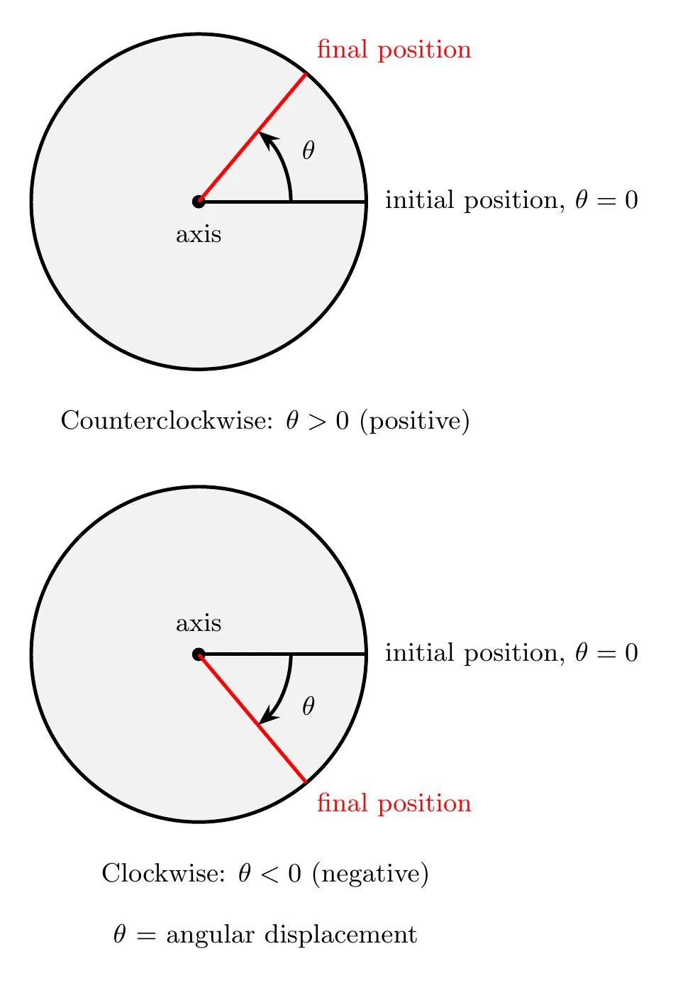
Compared to linear motion: - Linear displacement:

\Delta x

(meters). - Angular displacement:

\Delta \theta

(radians).

Angular Velocity

Angular velocity (

\omega

) is how fast the angular displacement changes with time.

\omega = \frac{d\theta}{dt}

Symbol:

\omega

(lowercase Greek omega). Units: rad/s.

Average angular velocity:

\omega_{avg} = \frac{\Delta \theta}{\Delta t}

Instantaneous angular velocity:

\omega = \lim_{\Delta t \to 0} \frac{\Delta \theta}{\Delta t} = \frac{d\theta}{dt}

The sign tells you: - Positive

\omega

: counterclockwise rotation. - Negative

\omega

: clockwise rotation. - Zero

\omega

: no rotation.

Compared to linear motion: - Linear velocity:

v = \frac{dx}{dt}

(m/s). - Angular velocity:

\omega = \frac{d\theta}{dt}

(rad/s).

Angular Acceleration

Angular acceleration (

\alpha

) is how fast the angular velocity changes with time.

\alpha = \frac{d\omega}{dt}

Symbol:

\alpha

(lowercase Greek alpha). Units: rad/s².

Average angular acceleration:

\alpha_{avg} = \frac{\Delta \omega}{\Delta t}

Instantaneous angular acceleration:

\alpha = \lim_{\Delta t \to 0} \frac{\Delta \omega}{\Delta t} = \frac{d\omega}{dt}

The sign tells you: - Positive

\alpha

: the angular velocity is increasing (speeding up, if rotating counterclockwise). - Negative

\alpha

: the angular velocity is decreasing (slowing down, if rotating counterclockwise).

Compared to linear motion: - Linear acceleration:

a = \frac{dv}{dt}

(m/s²). - Angular acceleration:

\alpha = \frac{d\omega}{dt}

(rad/s²).

Summary: The Calculus Relationships

Just like in linear kinematics, the rotational quantities connect through derivatives:

\theta \xrightarrow{\frac{d}{dt}} \omega \xrightarrow{\frac{d}{dt}} \alpha

Forward (differentiation):

\omega = \frac{d\theta}{dt} \quad \text{and} \quad \alpha = \frac{d\omega}{dt} = \frac{d^2\theta}{dt^2}

Backward (integration):

\omega = \int \alpha \, dt + \omega_0 \quad \text{and} \quad \theta = \int \omega \, dt + \theta_0

Example Problem: Angular Position as a Function of Time

Problem: A motor turns a disk back and forth. With counterclockwise as positive, the disk’s angular position is

\theta(t) = (0.50\text{ rad/s}^3)\,t^3 - (6.0\text{ rad/s})\,t

(a) Find

\omega(t)

and

\alpha(t)

. (b) When does the disk momentarily stop? (c) At

t = 1.0

s and at

t = 3.0

s, which way is the disk turning, and is it speeding up or slowing down? (d) Find the angular displacement from

t = 0

t = 3.0

s, and the total angle the disk turns through in that time.

Solution

(a) Differentiate. Angular velocity is the derivative of angular position, and angular acceleration is the derivative of angular velocity:

\omega(t) = \frac{d\theta}{dt} = (1.5\text{ rad/s}^3)\,t^2 - 6.0\text{ rad/s}

\alpha(t) = \frac{d\omega}{dt} = (3.0\text{ rad/s}^3)\,t

(b) Set the angular velocity to zero. Momentarily stopped means

\omega = 0

1.5t^2 - 6.0 = 0 \quad\Rightarrow\quad t^2 = 4.0 \quad\Rightarrow\quad t = 2.0\text{ s}

(c) Compare the signs. If

\omega

and

\alpha

have the same sign, the disk is speeding up. If they have opposite signs, it’s slowing down (just like

v

and

a

in Unit 1). - At

t = 1.0

\omega = 1.5(1.0)^2 - 6.0 = -4.5

rad/s (clockwise) and

\alpha = 3.0

rad/s² (counterclockwise). Opposite signs, so the disk is turning clockwise and slowing down. - At

t = 3.0

\omega = 1.5(3.0)^2 - 6.0 = 7.5

rad/s (counterclockwise) and

\alpha = 9.0

rad/s². Same sign, so it’s turning counterclockwise and speeding up.

(d) Integrate. The angular displacement is the integral of

\omega

\Delta\theta = \int_0^{3.0} \omega\,dt = \Big[0.50t^3 - 6.0t\Big]_0^{3.0} = 13.5 - 18.0 = -4.5\text{ rad}

The disk ends up 4.5 rad clockwise of where it started. But it reversed at

t = 2.0

s, so the total angle turned is bigger. Split the trip at the turnaround: - 0 to 2.0 s:

\theta(2.0) - \theta(0) = 4.0 - 12.0 = -8.0

rad (8.0 rad clockwise). - 2.0 to 3.0 s:

\theta(3.0) - \theta(2.0) = -4.5 - (-8.0) = +3.5

rad (3.5 rad counterclockwise). - Total angle turned:

8.0 + 3.5 = 11.5

rad, about 1.8 revolutions.

Angular displacement and total angle turned are different things, the same way displacement and distance were in Unit 1.

Linear vs. Angular Quantities

Linear (Translational)	Angular (Rotational)	Relationship
Position: $x$ (m)	Angular position: $\theta$ (rad)	$s = r\theta$
Velocity: $v$ (m/s)	Angular velocity: $\omega$ (rad/s)	$v = r\omega$
Acceleration: $a$ (m/s²)	Angular acceleration: $\alpha$ (rad/s²)	$a_t = r\alpha$

We’ll dig into those relationships (

s = r\theta

v = r\omega

a_t = r\alpha

) in the next topic.

Constant Angular Acceleration Kinematics Equations (CAKE)

When the angular acceleration is constant, you can use a set of kinematic equations that mirror the linear CAKE equations.

CAKE stands for Constant Angular Acceleration Kinematics Equations.

The Angular CAKE Equations

\omega_f = \omega_0 + \alpha t

\theta = \theta_0 + \omega_0 t + \frac{1}{2}\alpha t^2

\omega_f^2 = \omega_0^2 + 2\alpha(\theta - \theta_0)

\theta = \theta_0 + \frac{1}{2}(\omega_0 + \omega_f)t

where: -

\theta_0

= initial angular position (rad) -

\theta

= final angular position (rad) -

\omega_0

= initial angular velocity (rad/s) -

\omega_f

= final angular velocity (rad/s) -

\alpha

= angular acceleration (rad/s²), constant -

t

= time (s)

Comparison: Linear CAKE vs. Angular CAKE

Linear CAKE	Angular CAKE	What Changed?
$v_f = v_0 + at$	$\omega_f = \omega_0 + \alpha t$	$v \to \omega$ , $a \to \alpha$
$x = x_0 + v_0 t + \frac{1}{2}at^2$	$\theta = \theta_0 + \omega_0 t + \frac{1}{2}\alpha t^2$	$x \to \theta$ , $v \to \omega$ , $a \to \alpha$
$v_f^2 = v_0^2 + 2a(x - x_0)$	$\omega_f^2 = \omega_0^2 + 2\alpha(\theta - \theta_0)$	$v \to \omega$ , $a \to \alpha$ , $x \to \theta$
$x = x_0 + \frac{1}{2}(v_0 + v_f)t$	$\theta = \theta_0 + \frac{1}{2}(\omega_0 + \omega_f)t$	$x \to \theta$ , $v \to \omega$

The pattern is just a swap: -

x

(position) becomes

\theta

(angle). -

v

(velocity) becomes

\omega

(angular velocity). -

a

(acceleration) becomes

\alpha

(angular acceleration).

The structure of the equations is identical.

Example Problem: Saw Blade Spinning Down

Problem: A table saw blade spins at 524 rad/s (about 5000 rpm). When the saw is switched off, the blade slows down with a constant angular acceleration and stops in 3.20 s. (a) Find its angular acceleration. (b) How many revolutions does it make while stopping?

Solution

Take the blade’s direction of spin as positive, so

\omega_0 = +524

rad/s and

\omega_f = 0

. The angular acceleration is constant, so CAKE works.

(a) Use the equation without

\theta

\alpha = \frac{\omega_f - \omega_0}{t} = \frac{0 - 524\text{ rad/s}}{3.20\text{ s}} = -164\text{ rad/s}^2

The negative sign means

\alpha

points opposite to the spin, so the blade is slowing down.

(b) Use the equation without

\alpha

, so the rounding in (a) can’t creep in:

\Delta\theta = \tfrac{1}{2}(\omega_0 + \omega_f)t = \tfrac{1}{2}(524 + 0)(3.20) = 838\text{ rad}

\frac{838\text{ rad}}{2\pi\text{ rad/rev}} = 133\text{ rev}

Graphs in Rotational Kinematics

The same graphing principles from linear motion carry over to rotational motion.

Angular Velocity vs. Time Graph

For constant angular acceleration:

\omega = \omega_0 + \alpha t

That’s a linear function, so a straight line.

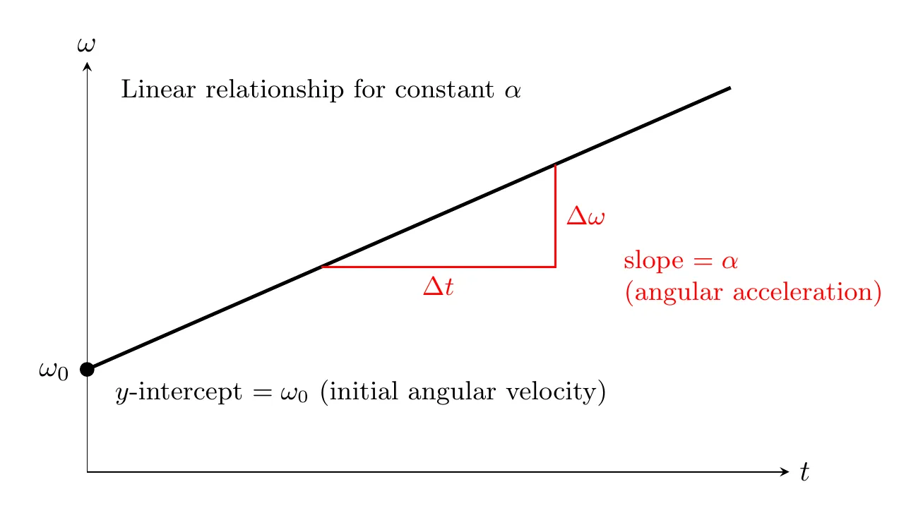
Angular Position vs. Time Graph

For constant angular acceleration:

\theta = \theta_0 + \omega_0 t + \frac{1}{2}\alpha t^2

That’s a quadratic function, so a parabola.

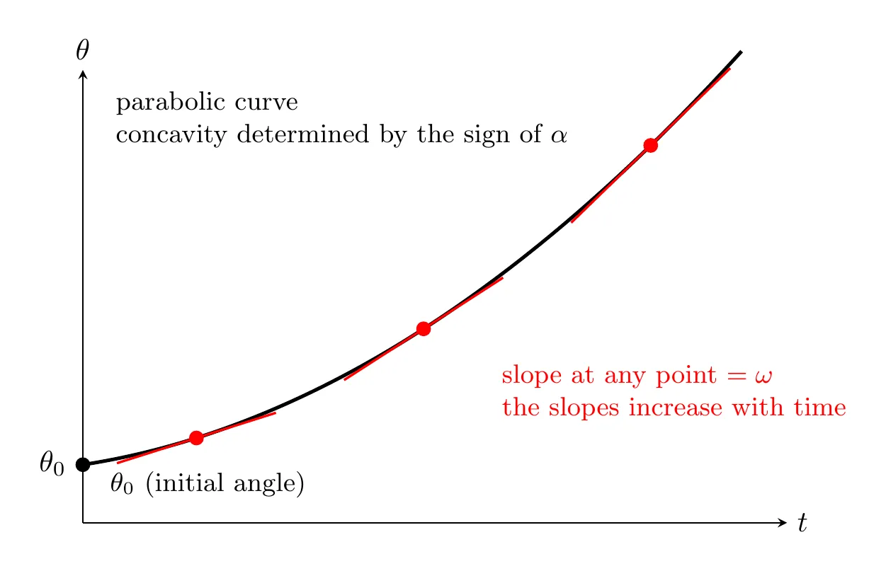
The interpretation is the same as in linear kinematics: - The slope of a

\theta

vs.

t

graph gives

\omega

. - The slope of an

\omega

vs.

t

graph gives

\alpha

. - The area under an

\omega

vs.

t

graph gives

\Delta \theta

. - The area under an

\alpha

vs.

t

graph gives

\Delta \omega

Example: Reading the Graphs

Problem: A lab turntable’s angular velocity is graphed in the middle panel below (counterclockwise positive,

\theta = 0

t = 0

). (a) Find the angular acceleration from 0 to 3.0 s and from 3.0 to 5.0 s. (b) When does the turntable reverse direction, and what is

\alpha

at that moment? (c) Find the angular displacement from 0 to 5.0 s and the total angle turned. (d) Sketch

\theta

vs.

t

and

\alpha

vs.

t

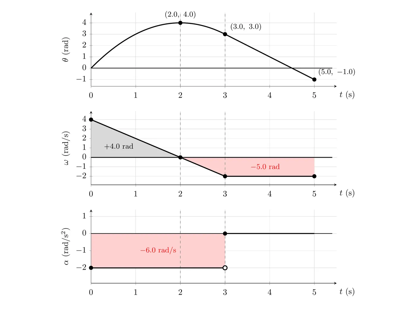
(a) The angular acceleration is the slope of the

\omega

vs.

t

graph:

\alpha = \frac{\Delta\omega}{\Delta t} = \frac{-2.0\text{ rad/s} - 4.0\text{ rad/s}}{3.0\text{ s} - 0} = -2.0\text{ rad/s}^2 \quad (0 \text{ to } 3.0\text{ s})

From 3.0 to 5.0 s the graph is flat, so

\alpha = 0

(b) The turntable reverses where

\omega

changes sign, at

t = 2.0

s. At that instant

\omega = 0

, but

\alpha

is still

-2.0

rad/s², because the slope of the line doesn’t change there. So the turntable slows down, reverses, and speeds up clockwise until the spin levels off at 2.0 rad/s at

t = 3.0

(c) The angular displacement is the signed area between the

\omega

graph and the time axis: - 0 to 2.0 s (triangle above the axis):

\frac{1}{2}(2.0)(4.0) = +4.0

rad. - 2.0 to 3.0 s (triangle below):

\frac{1}{2}(1.0)(-2.0) = -1.0

rad. - 3.0 to 5.0 s (rectangle below):

(2.0)(-2.0) = -4.0

rad.

\Delta\theta = 4.0 - 1.0 - 4.0 = -1.0\text{ rad} \qquad \text{total angle} = 4.0 + 1.0 + 4.0 = 9.0\text{ rad}

(d) Build each graph from the one you know: -

\theta

vs.

t

: its slope is

\omega

. From 0 to 3.0 s,

\alpha

is negative, so the curve is a downward-opening parabola. It peaks at

(2.0, 4.0)

, where

\omega = 0

(a flat tangent), and comes down to 3.0 rad at 3.0 s. From 3.0 to 5.0 s,

\omega

is a constant

-2.0

rad/s, so it’s a straight line with slope

-2.0

, ending at

-1.0

rad. -

\alpha

vs.

t

: a flat line at

-2.0

rad/s² from 0 to 3.0 s, then 0. Its area,

(3.0)(-2.0) = -6.0

rad/s, equals the change in

\omega

, from

+4.0

-2.0

rad/s.

Example Problem: Variable Angular Acceleration

Problem: A windmill is spinning at an initial angular speed

\omega_0

. A crosswind slows it down with an angular acceleration given by:

\alpha = -a\omega^2

where

a

is a positive constant. What is the windmill’s angular speed at time

t

Solution

Step 1: Recognize this needs calculus

The angular acceleration depends on the angular velocity (

\alpha = -a\omega^2

), so the constant acceleration equations are off the table. You have to use calculus.

Step 2: Write the relationship between $\alpha$ and $\omega$

\alpha = \frac{d\omega}{dt}

Step 3: Substitute the given expression

\frac{d\omega}{dt} = -a\omega^2

Step 4: Separate the variables

Rearrange so all the

\omega

terms are on one side and all the

t

terms are on the other:

\frac{d\omega}{\omega^2} = -a \, dt

or, equivalently:

\omega^{-2} d\omega = -a \, dt

Step 5: Integrate both sides

\int_{\omega_0}^{\omega} \omega'^{-2} \, d\omega' = \int_0^t (-a) \, dt'

Factor out the constant

-a

\int_{\omega_0}^{\omega} \omega'^{-2} \, d\omega' = -a \int_0^t dt'

Step 6: Evaluate the integrals

Left side, using the power rule

\int x^n dx = \frac{x^{n+1}}{n+1}

with

n = -2

\int \omega^{-2} d\omega = \frac{\omega^{-2+1}}{-2+1} = \frac{\omega^{-1}}{-1} = -\omega^{-1} = -\frac{1}{\omega}

Evaluate from

\omega_0

\omega

\left[-\frac{1}{\omega}\right]_{\omega_0}^{\omega} = -\frac{1}{\omega} - \left(-\frac{1}{\omega_0}\right) = -\frac{1}{\omega} + \frac{1}{\omega_0}

Right side:

-a \int_0^t dt' = -a[t']_0^t = -a(t - 0) = -at

Step 7: Set them equal

-\frac{1}{\omega} + \frac{1}{\omega_0} = -at

\frac{1}{\omega_0} - \frac{1}{\omega} = -at

Step 8: Solve for $\omega$

Rearrange:

\frac{1}{\omega} = \frac{1}{\omega_0} + at

Find a common denominator:

\frac{1}{\omega} = \frac{1 + \omega_0 at}{\omega_0}

Take the reciprocal:

\omega = \frac{\omega_0}{1 + \omega_0 at}

Answer: the angular speed at time

t

is:

\omega(t) = \frac{\omega_0}{1 + \omega_0 at}

The read: - At

t = 0

\omega = \omega_0

✓, so it starts at the initial speed. - As

t \to \infty

\omega \to 0

, so the windmill slows to a stop asymptotically. - The denominator grows with time, which drives

\omega

down. - The stronger the initial spin (

\omega_0

) or the stronger the resistance (

a

), the faster it slows.

When to Use Constant vs. Variable Acceleration

Use the CAKE equations when: - The angular acceleration is constant. - The problem says “uniform angular acceleration.” - No function is given for

\alpha

Use calculus when: - The angular acceleration varies with time:

\alpha(t)

. - It varies with position:

\alpha(\theta)

. - It varies with angular velocity:

\alpha(\omega)

, like the windmill problem. - You’re handed a function for any rotational quantity.

Common Mistakes

Mixing up linear and angular quantities. Don’t use $v$ in an angular equation or $\omega$ in a linear one. Keep them separate for now, since the next topic connects them.

Forgetting radians. Angular quantities must be in radians, not degrees. Convert with $\text{degrees} \times \frac{\pi}{180} = \text{radians}$ .

Getting the sign convention wrong. Counterclockwise is positive and clockwise is negative. Stay consistent through the whole problem.

Using CAKE when the acceleration isn’t constant. If $\alpha$ varies, you have to use calculus. The example problem shows exactly this.

Separating variables incorrectly. With $\frac{d\omega}{dt} = -a\omega^2$ , separate it into $\frac{d\omega}{\omega^2} = -a \, dt$ , not $d\omega = -a\omega^2 dt$ , which doesn’t actually separate the variables.

Integration errors with negative exponents. $\int \omega^{-2} d\omega = -\omega^{-1} = -\frac{1}{\omega}$ , not $+\frac{1}{\omega}$ . Watch your signs.

Not evaluating the limits properly. When you integrate from $\omega_0$ to $\omega$ , evaluate at the upper limit minus the lower limit.

Forgetting initial conditions. When you integrate, the constants of integration become your initial conditions. With definite integrals and proper limits, this gets handled automatically.

Confusing angular position with angular displacement. $\theta$ is the angular position and can be any value. $\Delta \theta = \theta - \theta_0$ is the angular displacement, the change in angle.

Taking the reciprocal wrong. If $\frac{1}{\omega} = \text{stuff}$ , then $\omega = \frac{1}{\text{stuff}}$ . Don’t invert it incorrectly.

Assuming the graphs are the same as the linear ones. The math forms are similar, but remember you’re plotting $\omega$ vs. $t$ or $\theta$ vs. $t$ , not $v$ vs. $t$ or $x$ vs. $t$ . The interpretation is rotational.

Not recognizing when a problem needs calculus. Key phrases: “varies with,” “depends on,” “is a function of,” or any time you’re handed an equation for $\alpha$ . Those all signal a calculus-based solution.

Unit errors. Angular velocity is rad/s, not m/s. Angular acceleration is rad/s², not m/s². Mixing these up breaks your dimensional analysis.

Thinking $\omega$ is a scalar. Angular velocity is actually a vector, with its direction set by the right-hand rule. But in problems with one axis of rotation, you can treat it as a scalar whose sign gives the direction.

Not checking the limiting cases. Always verify your answer makes sense at $t = 0$ (it should give the initial conditions) and as $t \to \infty$ (it should approach the expected behavior).

Back Next