4.1 - Electric Current

Introduction

Up to now you’ve been doing electrostatics, where charges shift around but don’t flow continuously. Now the focus turns to electric current, the continuous flow of charge through a conductor.

What Electric Current Is

Electric current is the rate at which charge passes through a cross-sectional area of a conductor:

I = \frac{dQ}{dt}

where: -

I

= electric current (A, amperes) -

Q

= charge (C) -

t

= time (s)

One ampere is one coulomb per second:

1 \text{ A} = 1 \text{ C/s}

Integral form. If you know current as a function of time, the total charge that moved through is:

Q = \int I \, dt

So current is the instantaneous rate of charge flow, and integrating it over time hands you the total charge transferred.

On the AP equation sheet this is

I = \frac{dq}{dt}

, with a lowercase

q

for the charge that has moved past. Same equation, different letter.

Example: The charge that has passed through a cross-section of a wire since

t = 0

q(t) = (3.0 \text{ C/s}^2)t^2 + (2.0 \text{ C/s})t

. Find the current at

t = 4.0

I = \frac{dq}{dt} = (6.0 \text{ C/s}^2)t + 2.0 \text{ C/s}

t = 4.0

I = (6.0)(4.0) + 2.0 = 26

Example: The current in a wire dies away as

I(t) = (5.0 \text{ A})e^{-t/(3.0 \text{ s})}

. How much charge passes a point in the wire during the first 3.0 s?

Q = \int_0^{3.0 \text{ s}} (5.0 \text{ A})e^{-t/(3.0 \text{ s})}\,dt = (5.0 \text{ A})(3.0 \text{ s})\left[-e^{-t/(3.0 \text{ s})}\right]_0^{3.0 \text{ s}} = (15 \text{ C})\left(1 - e^{-1}\right)

That’s

Q = (15 \text{ C})(0.632) = 9.5

C. Let the integral run all the way to

t \to \infty

and you get the total, 15 C: the whole area under the

I

vs.

t

curve.

Current in Terms of Drift Velocity

You can also write current in terms of how the charge carriers (electrons) actually move:

I = nqv_d A

where: -

n

= number density of charge carriers (charges per unit volume, m⁻³) -

q

= charge on each carrier (C); for electrons,

q = e = 1.6 \times 10^{-19}

C -

v_d

= drift velocity (average velocity of the carriers, m/s) -

A

= cross-sectional area of the conductor (m²)

Drift velocity (

v_d

) is the average speed at which charge carriers creep through the conductor in response to an electric field. Here’s the surprising part: individual electrons are zipping around extremely fast (close to

10^6

m/s) in random directions, but their net drift down the wire is slow, typically a fraction of a millimeter per second, because they’re constantly colliding with atoms.

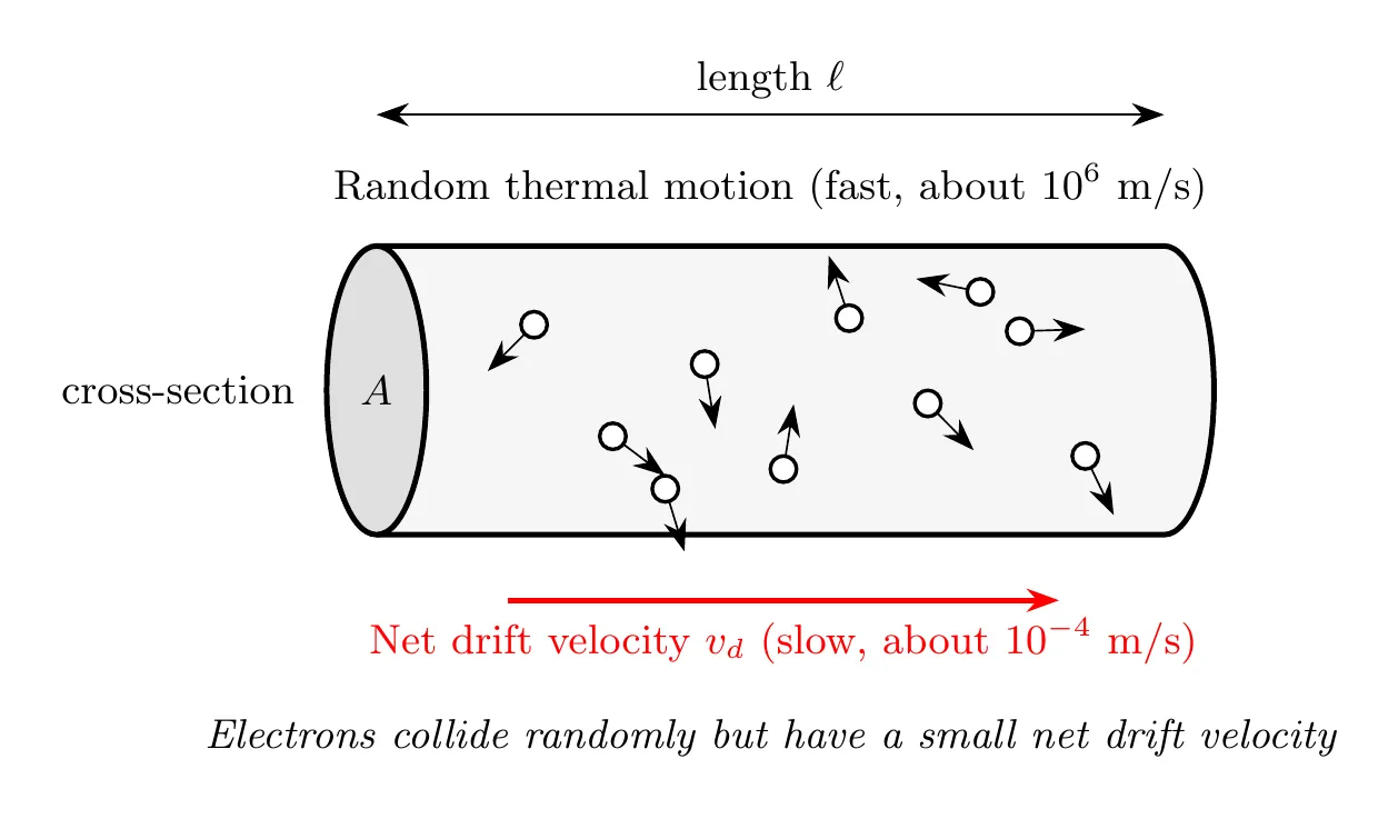
Where $I = nqv_dA$ comes from. It isn’t on the equation sheet, but it only takes a few lines to build. Picture the carriers drifting along a wire of cross-sectional area

A

. In a short time

dt

, each one moves a distance

v_d\,dt

, so every carrier inside a slice of length

v_d\,dt

crosses the end of that slice. The slice has volume

Av_d\,dt

, so it holds

nAv_d\,dt

carriers, each with charge

q

dq = q\,(nAv_d\,dt) \quad\Rightarrow\quad I = \frac{dq}{dt} = nqv_dA

Example: A copper wire with a radius of 1.0 mm carries a 2.0 A current. Copper has about

8.5 \times 10^{28}

free electrons per cubic meter. Find the drift speed.

v_d = \frac{I}{nqA} = \frac{2.0 \text{ A}}{(8.5 \times 10^{28} \text{ m}^{-3})(1.60 \times 10^{-19} \text{ C})\pi(1.0 \times 10^{-3} \text{ m})^2} = 4.7 \times 10^{-5} \text{ m/s}

That’s about 0.05 mm/s. At that pace, an electron takes almost 6 hours to drift 1 m down the wire.

Zero current doesn’t mean the electrons are sitting still. In a wire with no current, the free electrons still race around at about

10^6

m/s. Their directions are random, though, so just as many cross any cross-section going one way as going the other. Their average velocity is zero, so the net flow of charge (the current) is zero. A potential difference doesn’t make the electrons fast. It adds a tiny average drift on top of motion they already have.

Electric Potential Difference and EMF

Charge moves through a circuit because of a potential difference (voltage).

EMF (electromotive force, written

\mathcal{E}

) is the voltage supplied by a source like a battery or generator. Despite the name, EMF is not a force. It’s a potential difference measured in volts.

There’s a distinction worth keeping straight. The EMF (

\mathcal{E}

) is the ideal voltage the source wants to provide, while the terminal voltage (

V

) is the actual voltage across the terminals once current is flowing, which is usually a bit less because of internal resistance. That gap gets explored properly in a later topic.

How the potential difference moves the charge. The battery keeps one end of the circuit at a higher potential than the other. That potential difference sets up an electric field inside the wires and the other elements, pointing from high potential toward low potential, and the field pushes the charge carriers along. No potential difference across an element means no field inside it, so no current through it, no matter how good a conductor it is.

Example: Connect a 3.0 Ω resistor across a 1.5 V battery and the battery drives

I = \frac{\Delta V}{R} = \frac{1.5}{3.0} = 0.50

A through it (Ohm’s law, coming up in topic 4.3). Now connect both ends of the same resistor to the battery’s positive terminal. Both ends sit at the same potential, so

\Delta V = 0

and

I = 0

, even though the battery is still right there.

Current Density

Current density describes how the current spreads across the cross-section, essentially current per unit area:

J = \frac{I}{A}

where

J

is the current density (A/m²),

I

is the total current (A), and

A

is the cross-sectional area (m²).

In terms of the charge carriers:

J = nqv_d

which is just the current-density version of

I = nqv_d A

. Rearranging the definition gives

I = JA

. Conceptually, current density works a lot like flux: it describes flow per unit area rather than total flow.

Current density is a vector.

\vec{J}

points in the direction positive charge flows at that spot (the conventional current direction), and its magnitude is the current per unit area there. In vector form:

\vec{J} = nq\vec{v}_d

For electrons,

q = -e

is negative, so

\vec{J}

points opposite to the electrons’ drift velocity, which is exactly the conventional current direction. Current itself isn’t a vector (more on that below), but current density is, because it describes the flow at each point in the conductor.

Example: The 2.0 A copper wire from the drift velocity example (radius 1.0 mm) has

J = \frac{I}{A} = \frac{2.0 \text{ A}}{\pi(1.0 \times 10^{-3} \text{ m})^2} = 6.4 \times 10^5

A/m², pointing along the wire in the direction of the conventional current.

Resistivity and Electric Field

The electric field inside a conductor connects to the current density through the material’s resistivity:

E = \rho J

where: -

E

= electric field in the conductor (V/m) -

\rho

(rho) = resistivity of the material (Ω·m) -

J

= current density (A/m²)

Careful here: this

\rho

is resistivity, a material property, not the volume charge density from earlier units. You have to read the context to know which one you’re looking at.

What it means physically: for a given current density, a material with higher resistivity builds up a stronger electric field, because it fights the current harder. Resistivity is the material property that leads into the idea of resistance, which comes up with Ohm’s law shortly.

On the AP equation sheet this is a vector equation,

\vec{E} = \rho\vec{J}

, so the field inside the conductor points the same way as the current density. The potential difference across the conductor is what creates that field: for a uniform wire of length

L

with potential difference

\Delta V

across it,

E = \frac{\Delta V}{L}

This doesn’t contradict Unit 3. The field inside a conductor is zero only in electrostatic equilibrium, when no charge is moving. Once there’s a current, a small field inside the conductor keeps pushing the carriers along. Example: for the same 2.0 A copper wire (

\rho = 1.7 \times 10^{-8}

Ω·m):

E = \rho J = (1.7 \times 10^{-8}\ \Omega\cdot\text{m})(6.4 \times 10^5 \text{ A/m}^2) = 1.1 \times 10^{-2} \text{ V/m}

Across 1.0 m of this wire, the potential drops only about 0.011 V, which is why you can usually ignore the wires in a circuit (topic 4.5).

Current from a Current Density Function

When the current density isn’t uniform across the cross-section, you have to integrate to get the total current:

I = \int \vec{J} \cdot d\vec{A}

For problems with cylindrical symmetry, where

J

depends only on the radial distance

r

from the axis, this becomes

I = \int J \, dA

. For a circular cross-section, the area element in polar coordinates is:

dA = 2\pi r \, dr

so:

I = \int_0^R J(r) \cdot 2\pi r \, dr

where

R

is the conductor’s radius.

Conventional Current vs. Electron Flow

Current has a direction, even though current itself is technically a scalar.

Conventional current is defined as the direction positive charges would flow: from the positive terminal, through the circuit, to the negative terminal. This convention was locked in before anyone knew electrons existed.

Actual electron flow in metal conductors goes the other way, since the real carriers are electrons (negative): they travel from the negative terminal, through the circuit, to the positive terminal. So electron flow runs opposite to conventional current.

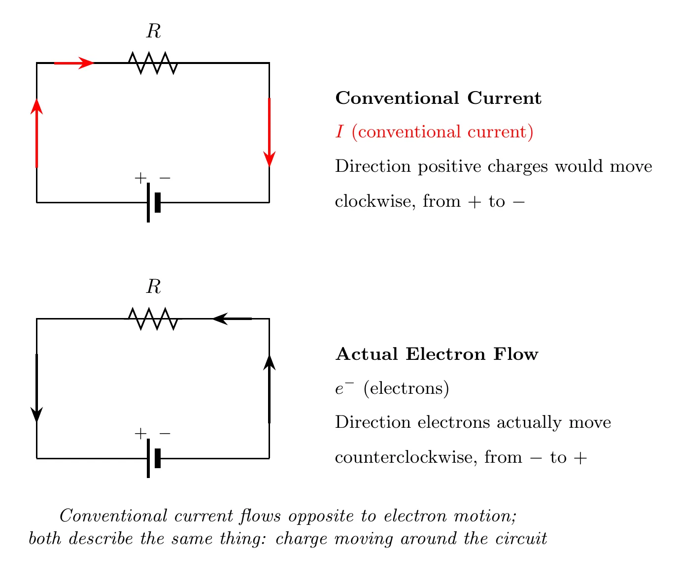
Why bother with conventional current? It’s historical (set before the electron was discovered), the math works out identically either way, and positive current in one direction is the same as negative charge flowing the other direction. In practice, circuit analysis almost always uses conventional current.

Current has a direction, but it isn’t a vector. The direction of a current is along the wire, relative to the wire itself, not a fixed direction in space. Bend the wire around a corner and the current is the same before and after the bend. So currents don’t follow the rules of vector addition and don’t have x- and y-components. At a junction, you just add them as numbers. (Current density

\vec{J}

, on the other hand, is a vector.)

Example: A wire carrying 3.0 A and a wire carrying 4.0 A meet at a right angle and join into a third wire. The third wire carries

3.0 + 4.0 = 7.0

A. Adding them like vectors would give

\sqrt{3.0^2 + 4.0^2} = 5.0

A, which can’t be right: 2.0 C of charge would vanish at the junction every second.

Example Problem: Current in a Cylindrical Conductor

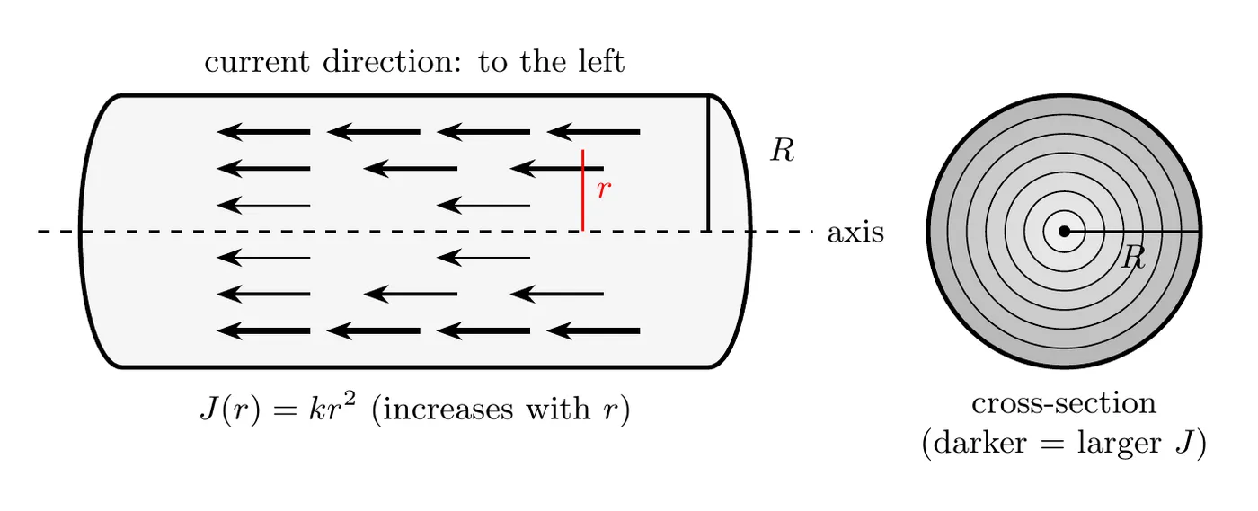
A long conducting cylinder of radius

R

carries a current to the left. The current density varies with distance

r

from the central axis as:

J(r) = kr^2

for

r \leq R

, where

k

is a positive constant. Derive an expression for the total current in terms of

k

and

R

Solution

Set up the integral. With a non-uniform current density, the total current is the integral of

J

over the cross-sectional area:

I = \int \vec{J} \cdot d\vec{A}

Pick the right area element. With cylindrical symmetry, use a thin ring at radius

r

with thickness

dr

, whose area is its circumference times its thickness:

dA = 2\pi r \, dr

Build the integral using

J(r) = kr^2

I = \int_0^R kr^2 \cdot 2\pi r \, dr = \int_0^R 2\pi k r^3 \, dr = 2\pi k \int_0^R r^3 \, dr

Integrate with the power rule, since

\int r^3 \, dr = \frac{r^4}{4}

I = 2\pi k \left[\frac{r^4}{4}\right]_0^R = 2\pi k \cdot \frac{R^4}{4} = \frac{\pi k R^4}{2}

So the total current is

I = \frac{\pi k R^4}{2}

Reading the result: the current scales with

R^4

, a fourth power, because both the area and the current density grow as you move outward. And a bigger

k

means a higher current density everywhere, so proportionally more total current.

Example Problem: Current Density That Falls Off Outward

A wire of radius

R = 2.0

mm has a current density that is largest on its axis and drops to zero at its surface:

J(r) = J_0\left(1 - \frac{r}{R}\right)

with

J_0 = 3.0 \times 10^6

A/m². Find (a) the total current in the wire and (b) the current within

r < \frac{R}{2}

Solution

(a) Set up the same ring integral as the example above, with

dA = 2\pi r\,dr

I = \int_0^R J_0\left(1 - \frac{r}{R}\right)2\pi r\,dr = 2\pi J_0\left[\frac{r^2}{2} - \frac{r^3}{3R}\right]_0^R = 2\pi J_0\left(\frac{R^2}{2} - \frac{R^2}{3}\right) = \frac{\pi J_0 R^2}{3}

I = \frac{\pi(3.0 \times 10^6 \text{ A/m}^2)(2.0 \times 10^{-3} \text{ m})^2}{3} = 13 \text{ A}

(b) Same integral, smaller upper limit. Stop at

r = \frac{R}{2}

I_{inner} = 2\pi J_0\left[\frac{r^2}{2} - \frac{r^3}{3R}\right]_0^{R/2} = 2\pi J_0\left(\frac{R^2}{8} - \frac{R^2}{24}\right) = \frac{\pi J_0 R^2}{6} = 6.3 \text{ A}

Half the current flows inside

r < \frac{R}{2}

, even though that’s only a quarter of the cross-sectional area, because the current density is biggest near the axis. Compare the example above, where

J

grows outward and most of the current crowds near the surface.

Summary of Current Formulas

Expression	Formula	When to use
Definition	$I = \frac{dQ}{dt}$	Rate of charge flow
Integrated charge	$Q = \int I \, dt$	Total charge from current
Drift velocity form	$I = nqv_dA$	Relating to charge carrier motion
Current density	$J = \frac{I}{A}$ or $J = nqv_d$	Current per unit area
From density	$I = JA$	Uniform current density
Non-uniform density	$I = \int J \, dA$	Varying current density
Field and resistivity	$E = \rho J$	Relating field to current

On the AP equation sheet:

I = \frac{dq}{dt}

I = \int \vec{J} \cdot d\vec{A}

, and

\vec{E} = \rho\vec{J}

. The drift velocity forms,

I = nqv_dA

and

\vec{J} = nq\vec{v}_d

, aren’t on the sheet, so know where they come from.

Current Direction Convention

Convention	Flow direction	Reality
Conventional current	From + to −	What we use in circuit analysis
Electron flow	From − to +	What physically happens in metals

Both describe the same physics. Conventional current is just defined opposite to the actual electron motion.

Typical Drift Velocities

To get a feel for how slow drift velocity really is: a household wire carrying 1 A has a drift velocity around 0.1 mm/s, a nerve impulse travels around 100 m/s (though that’s signal speed, not drift), and the random thermal motion of electrons runs around

10^6

m/s.

So why do lights turn on instantly? Because the electric field propagates through the wire at nearly the speed of light (about

3 \times 10^8

m/s), even though the individual electrons barely crawl. Think of a pipe already full of water: push on one end and water comes out the other end immediately, even though any single water molecule takes forever to travel the length of the pipe.

Common Mistakes

Confusing current with current density. Current $I$ is the total charge flow (amperes). Current density $J$ is current per unit area (A/m²). They’re not interchangeable in formulas.

Thinking drift velocity is fast. It’s typically very slow (a fraction of a millimeter per second), even though the field propagates almost instantly. Don’t mix up drift velocity with signal speed or with the electrons’ random thermal velocity.

Mixing up the two meanings of $\rho$ . It can mean volume charge density (C/m³) or resistivity (Ω·m) depending on context. In current problems it usually means resistivity. Check the units.

Forgetting the area element in cylindrical coordinates. Integrating over a circular cross-section, the area element is $dA = 2\pi r \, dr$ , not just $dr$ and not $\pi r^2$ . It accounts for the circumference at radius $r$ .

Using the wrong current direction. Default to conventional current (positive charge flow, + to −) unless you’re specifically told otherwise.

Adding currents like vectors. Current has a direction along the wire, but it isn’t a vector. At a junction, currents add as plain numbers, whatever the angle between the wires.

Back Next