

1.6 - Marginal Analysis and Consumer Choice
This section covers marginal analysis, the Law of Diminishing Marginal Utility, the utility-maximization formula, and how to find the benefit-maximizing quantity where marginal benefit meets or exceeds marginal cost.
Thinking at the margin
Most economic decisions aren’t all-or-nothing, they happen “at the margin,” meaning we look at the impact of just the next unit.
Marginal is calculated as the change in total divided by the change in quantity: . Since quantity usually changes by one unit at a time, you can often just look at the difference between totals.
- If the total is rising at a decreasing rate, the marginal value is positive but falling.
- If the total is decreasing, the marginal value is negative.
- Total utility peaks exactly when marginal utility hits zero.
Marginal benefit vs. marginal cost
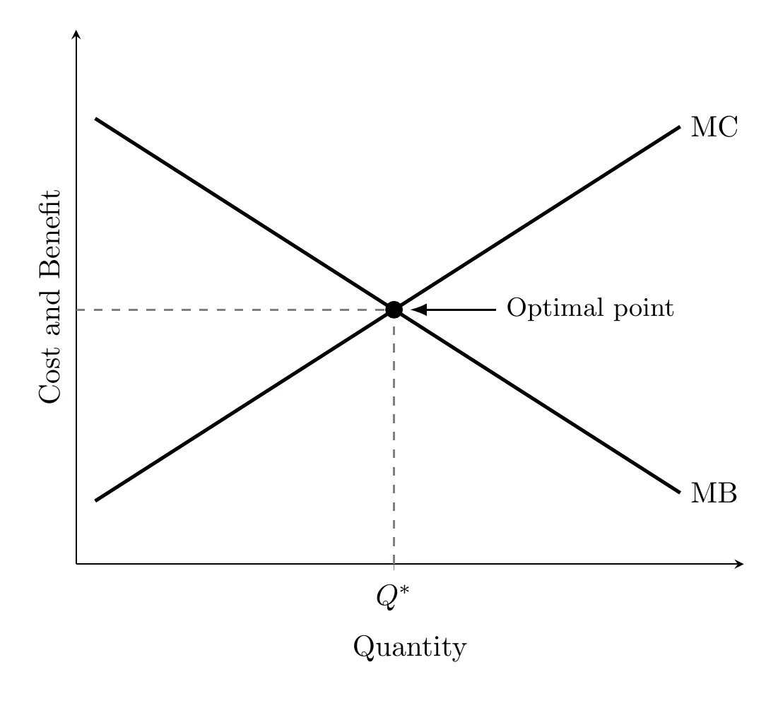
- Marginal benefit (MB): the extra satisfaction from one more unit. Spend an extra hour practicing a skill, and MB is the specific boost in your performance from that hour alone. MB curves slope downward since each extra unit usually adds less value than the last.
- Marginal cost (MC): the extra cost of one more unit. Staying at the gym an extra hour costs you more than physical effort, it costs you the sleep or social time you gave up. MC curves slope upward because resources like time get scarcer and more valuable the more you use them.
The benefit-maximization rule
Keep going as long as . If MB is $20 and MC is $15 for a unit, that unit adds $5 to your total satisfaction. You stop the moment the next unit’s MC would exceed its MB, and that’s where total net benefit peaks.
Put another way, compare the marginal benefit and marginal cost of the next unit:
- : do more, since the next unit adds more benefit than cost.
- : do less, since the last unit cost more than it was worth.
- : stay put. This is the optimal quantity, where the MB and MC curves cross on the graph above and total net benefit is maximized.
Firms use the same logic to decide how much to produce. In Unit 3 it becomes the rule “produce where marginal revenue equals marginal cost.”
Ignore sunk costs
The optimal quantity only depends on what happens from here on. Fixed costs or fixed benefits already locked in by past choices (sunk costs) don’t change the MB or MC of the next unit, so they shouldn’t change your decision. At an all-you-can-eat buffet, the $20 you paid at the door is sunk. Whether you go back for another plate should depend only on how much you’d enjoy it (MB) versus how stuffed you’d feel (MC), not on “getting your money’s worth.”
Key assumptions of consumer choice
Consumer choice theory, the model for how people decide what to buy, rests on a few assumptions:
- Consumers are rational: they make choices to get the most total utility (satisfaction) they can.
- Consumers face constraints: income is limited and prices are set, so they can’t buy everything. Every choice has to fit inside the budget.
- Marginal utility diminishes: each extra unit of a good adds less satisfaction than the one before (more on this below).
Diminishing marginal utility
Utility is just the satisfaction a consumer gets from a product, and the extra satisfaction from each additional unit shrinks as you consume more. Your first coffee of the day feels amazing, the second is good but less exciting, and by cup six you might actually feel worse, meaning marginal utility has gone negative.
Maximizing utility on a budget
You’ve maximized utility when the marginal utility per dollar is equal across everything you buy:
If one item gives you more “utils per dollar” than another, buy more of it and less of the other, it’s a better value for your limited budget. In practice you spend your budget one unit at a time, always picking whatever gives you the highest marginal utility per dollar at that moment.
Worked example: maximizing utility
Jada has $8 to spend on pizza slices ($2 each) and sodas ($1 each). Her marginal utility from each unit is below. First divide each MU by the price to get MU per dollar:
Unit | MU of pizza | MU per dollar (pizza) | MU of soda | MU per dollar (soda) |
1st | 20 | 10 | 8 | 8 |
2nd | 16 | 8 | 6 | 6 |
3rd | 12 | 6 | 4 | 4 |
4th | 8 | 4 | 3 | 3 |
5th | 4 | 2 | 2 | 2 |
Then spend the budget on whatever gives the most MU per dollar at each step:
- 1st pizza slice (10 per dollar beats 8 for soda). Total spent: $2.
- 2nd pizza slice and 1st soda (tied at 8 per dollar). Total spent: $5.
- 3rd pizza slice and 2nd soda (tied at 6 per dollar). Total spent: $8, so the budget is gone.
Jada’s best choice is 3 pizza slices and 2 sodas. Check both rules: she spends exactly $8 (3 slices at $2 plus 2 sodas at $1), and the last unit of each good gives the same MU per dollar ( for the 3rd slice, for the 2nd soda). Her total utility is utils, more than any other combination she can afford (4 slices and no soda give 56, and 2 slices and 4 sodas give 57).
Takeaway
Marginal analysis is the zoom lens of economic decisions, it focuses on the value of the very next step rather than the big picture. Life is a series of tiny trade-offs where we’re constantly weighing the extra gain against the extra sacrifice, chasing the sweet spot where satisfaction peaks before diminishing returns kick in.