

3.2 - Short-Run Production Costs
This covers fixed, variable, and total costs, the graphical relationship between marginal and average cost curves, and how taxes or subsidies shift these cost structures.
Categorizing short-run costs
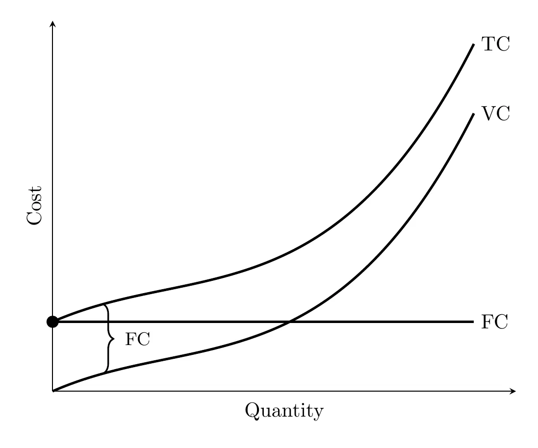
- Fixed costs (FC): stay the same no matter how much you produce, often called overhead. Examples: a monthly lease on a pizza oven, loan interest payments, a security guard’s salary.
- Fixed costs are the same at every output level, including zero output. A firm that makes nothing still owes them, so at , .
- Variable costs (VC): change directly with output, and are zero if production is zero. Examples: flour and cheese for a bakery, hourly wages for seasonal staff, electricity for machinery.
- Total cost (TC): fixed plus variable costs (including both implicit and explicit) at a given output level.
Marginal cost
Marginal cost is the change in total cost from producing one more unit: . Since quantity usually increases one at a time, it’s basically the cost increase for that next unit.
MC first decreases due to specialization, then eventually increases due to diminishing marginal returns.
Why that shape: if labor is the only variable input, . At first, specialization and the division of labor raise each worker’s marginal product, so each extra unit takes less labor and MC falls. Once diminishing marginal returns set in, marginal product falls, so each extra unit takes more labor and MC rises. That’s why a production function with diminishing marginal returns gives an upward-sloping MC curve.
Since fixed costs don’t change with output, MC is also the change in variable cost: .
The average cost family
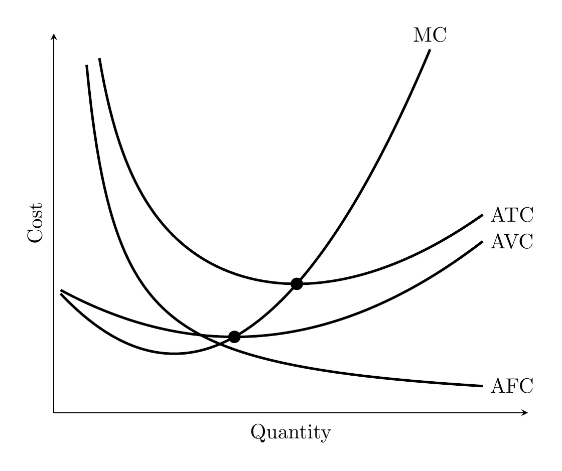
- Average fixed cost (AFC): fixed cost divided by quantity. Always falls as output rises, since the same overhead spreads across more units.
- Average variable cost (AVC): variable cost divided by quantity.
- Average total cost (ATC): total cost divided by quantity, or AFC plus AVC.
- As output rises: AFC keeps falling. AVC and ATC are U-shaped: they fall at first (specialization, and for ATC, fixed costs spread over more units), then rise (diminishing marginal returns).
- The gap between ATC and AVC is AFC. Since AFC shrinks as output grows, ATC and AVC get closer together at higher output, but never touch. And since ATC sits above AVC, the rising MC curve reaches the bottom of AVC first, so the lowest point of ATC is always to the right of the lowest point of AVC.
Productive efficiency happens at the minimum point of ATC, where , the lowest possible per-unit cost.
The intersection rule
Marginal cost always crosses AVC and ATC exactly at their minimum points. If the “next unit” costs less than the average, the average falls. If it costs more, the average rises.
Calculating costs from a table
A small T-shirt shop pays $12 a day in fixed costs (rent on its printer). All numbers are in dollars.
Output (Q) | FC | VC | TC | MC | AFC | AVC | ATC |
0 | 12 | 0 | 12 | ||||
1 | 12 | 8 | 20 | 8 | 12 | 8 | 20 |
2 | 12 | 11 | 23 | 3 | 6 | 5.50 | 11.50 |
3 | 12 | 15 | 27 | 4 | 4 | 5 | 9 |
4 | 12 | 21 | 33 | 6 | 3 | 5.25 | 8.25 |
5 | 12 | 28 | 40 | 7 | 2.40 | 5.60 | 8 |
6 | 12 | 39 | 51 | 11 | 2 | 6.50 | 8.50 |
- TC = FC + VC. At 4 shirts: $12 + $21 = $33.
- MC is the change in TC. Going from 3 to 4 shirts, TC rises from $27 to $33, so MC = $6. MC falls at first (specialization), bottoms out at the 2nd shirt, then rises (diminishing marginal returns).
- Each average is a total divided by Q. At 4 shirts: AFC = 12 / 4 = $3, AVC = 21 / 4 = $5.25, and ATC = 33 / 4 = $8.25 (which also equals AFC + AVC).
- MC crosses the averages at their lowest points. AVC bottoms out at $5 (3 shirts): the next shirt’s MC ($6) is above it, so AVC starts rising. ATC bottoms out at $8 (5 shirts): the next shirt’s MC ($11) is above it, so ATC starts rising.
Shifting cost curves
- Lump-sum changes (a one-time tax, subsidy, or rent change): only shifts ATC and AFC up or down, doesn’t touch marginal cost since it doesn’t change the cost of the next unit.
- Per-unit changes (a tax or subsidy on every item, or a change in raw material prices): shifts MC, AVC, and ATC all at once.
- Productivity changes work like per-unit changes: if workers or machines get more productive (better technology or training), each unit takes fewer inputs, so MC, AVC, and ATC all shift down. A drop in productivity, or a higher wage, shifts them up. AFC doesn’t move, since fixed costs stay the same.
Takeaway
A firm’s cost structure comes from the interplay of fixed overhead and variable inputs. Fixed costs stay put, but diminishing returns eventually push marginal and average costs upward. Productive efficiency means producing right where marginal cost equals average total cost, the lowest cost per unit possible.