

3.3 - Long-Run Production Costs
This covers the difference between short-run and long-run cost structures, how the Long Run Average Total Cost (LRATC) curve is derived, and what causes economies and diseconomies of scale.
Defining the long run
- Short run: at least one input (usually plant size) is fixed. A firm can vary its production rate with variable inputs like labor, but capacity is capped.
- Long run: all inputs are variable. A firm can change both production rate and total capacity by building new facilities or buying more equipment.
- Since every input can change, all costs are variable in the long run. There are no fixed costs, because even the building or the lease can be changed or dropped.
The LRATC curve
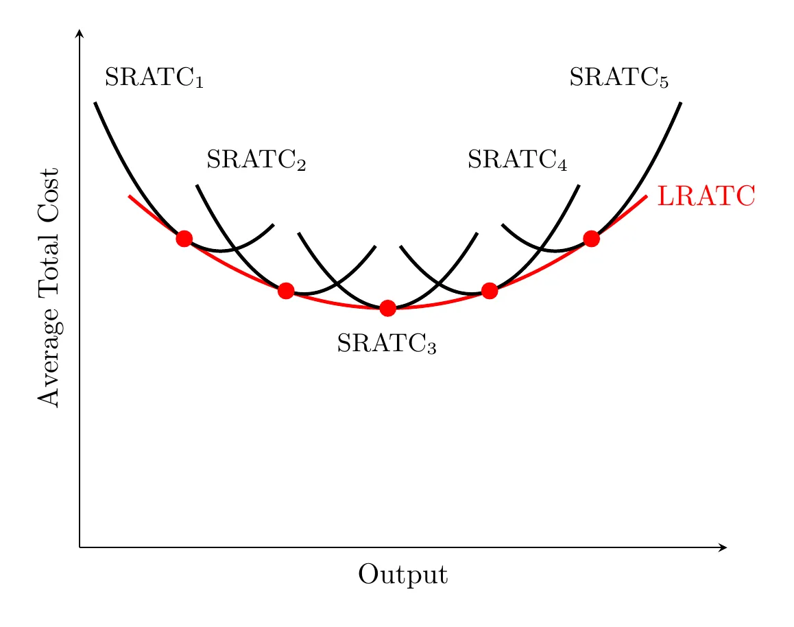
A firm’s long-run costs are basically a collection of different short-run options. Every possible plant size has its own Short Run Average Total Cost (SRATC) curve, and the LRATC curve is the envelope that just touches each of those curves from below. It represents the lowest possible average cost for any output level, once a firm is free to pick its plant size.
Phases of long-run production
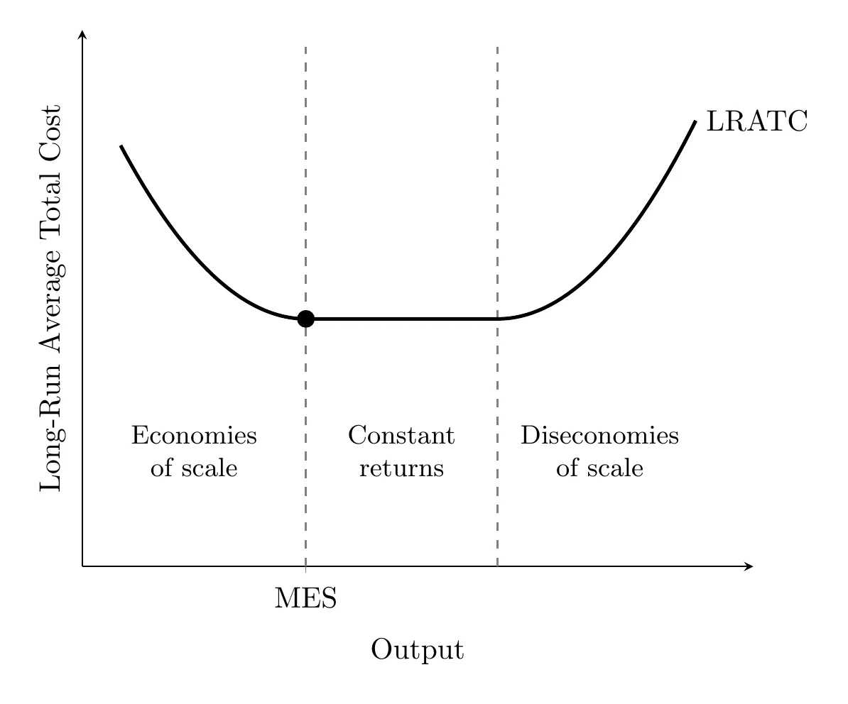
- Economies of scale: LRATC slopes downward, average costs fall as the firm expands. This happens because larger firms get bulk discounts on materials, can afford advanced tech or specialized machinery, and benefit from specialized management. A small furniture maker buying wood at retail and using hand tools might, after scaling up into a big factory, buy lumber at a steep discount and use automated assembly lines that cut cost per chair way down.
- Constant returns to scale: LRATC flattens out, average costs stay the same as capacity grows. The minimum efficient scale (MES) is the lowest output level where a firm minimizes its long-run average cost, and in a competitive market, firms generally need to hit at least this scale to stay viable.
- Diseconomies of scale: LRATC slopes upward, average costs rise as the firm grows too large, usually from bureaucratic bloat, communication breakdowns, and the sheer difficulty of managing a massive workforce. The business gets too top-heavy to run efficiently.
Minimum efficient scale and market structure
Where the MES falls compared to the size of the whole market helps decide how many firms the market can hold:
- Small MES (reached at an output that’s tiny compared to market demand): lots of firms can each reach the lowest long-run cost, so the market can support many competitors. Think restaurants, hair salons, or farms.
- Large MES (only reached at an output that’s a big share of market demand): only a few firms can produce at a low cost, and small firms can’t keep up. The market ends up concentrated, like an oligopoly (car makers, airplane makers). If economies of scale continue across the whole market, one firm can supply everyone at the lowest cost, which is a natural monopoly (like a local electric grid).
Returns to scale, the math
This compares the percentage change in all inputs to the percentage change in output.
- Increasing returns to scale: double all inputs and output more than doubles. This creates the downward-sloping economies of scale portion of the curve.
- Constant returns to scale: double all inputs, output exactly doubles. This matches the flat portion of LRATC.
- Decreasing returns to scale: double all inputs, output less than doubles. This creates the upward-sloping diseconomies of scale portion.
- Example: a firm doubles all its inputs (workers, machines, and space) at the same input prices, so its long-run total cost doubles from $1,000 to $2,000. If output goes from 100 to 250 units, that’s increasing returns to scale, and long-run ATC falls from $1,000 / 100 = $10 to $2,000 / 250 = $8 (economies of scale). If output exactly doubles to 200, ATC stays at $10 (constant returns). If output only rises to 160, ATC rises to $2,000 / 160 = $12.50 (decreasing returns, diseconomies of scale).
- Don’t mix these up with diminishing marginal returns. Diminishing marginal returns is a short-run idea: one input grows while the others stay fixed (3.1). Returns to scale and economies or diseconomies of scale are long-run ideas: all inputs grow together.
Takeaway
In the long run, firms can adjust their entire scale of operations. Expansion typically brings economies of scale at first, with specialization and bulk buying driving per-unit costs down. But grow too large, and diseconomies of scale can set in from management complexity, pushing costs back up. Most firms aim to reach the minimum efficient scale to stay competitive.