3.7 - Perfect Competition

Characteristics

A perfectly competitive market has specific traits that keep any single firm from influencing price:

Many sellers: lots of small firms competing.

Standardized products: goods are identical, no brand differences. Think Grade A large white eggs, one farm’s egg is indistinguishable from another’s.

Low barriers to entry/exit: easy to start up or leave.

In the model there are no real barriers: no patents, licenses, or huge startup costs keep new firms out. That’s what lets entry and exit wipe out profits and losses in the long run.

Price takers: with identical products and tons of sellers, no individual firm can set its own price. Everyone accepts the market’s equilibrium price.

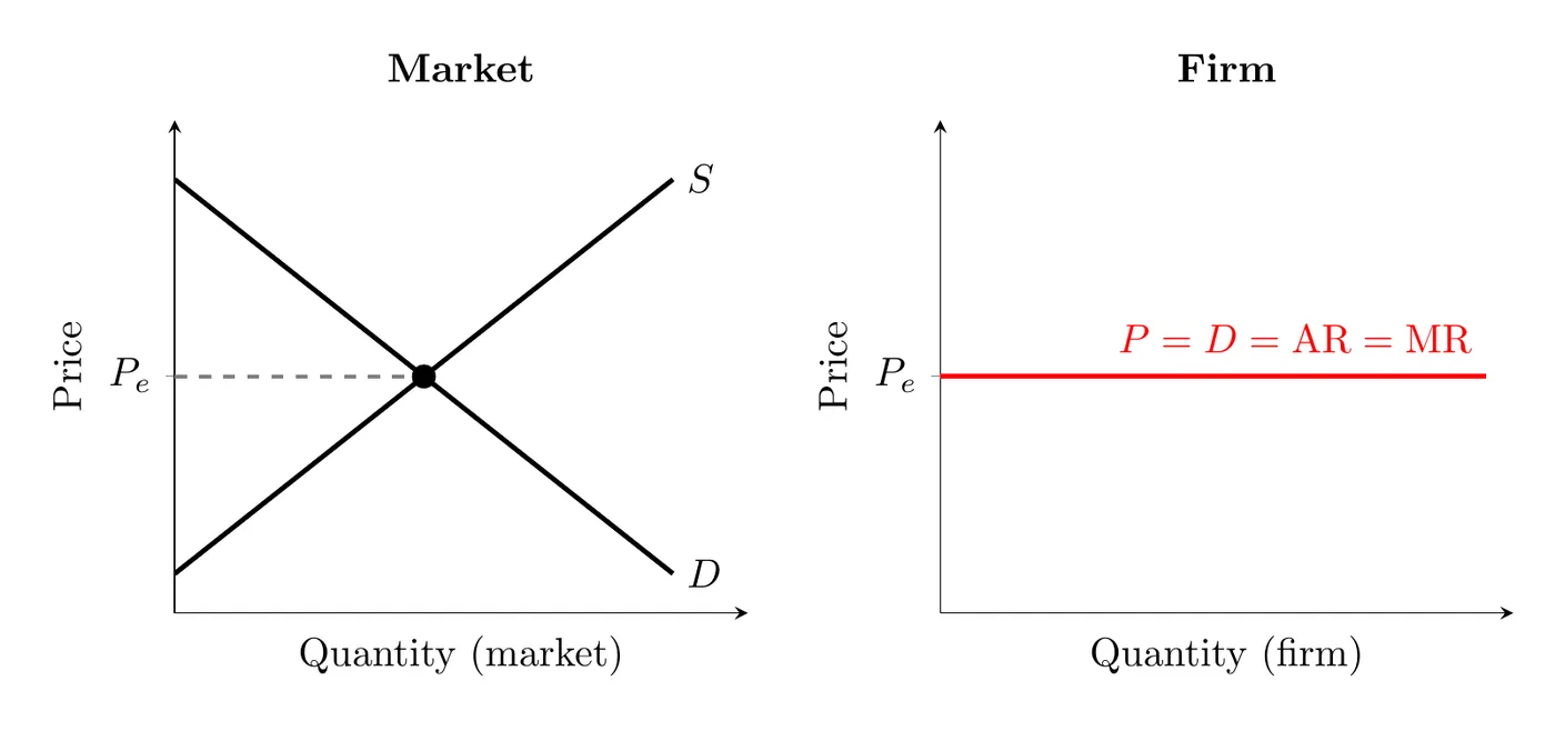
This means each firm has no market power. If one egg farm charged even a penny above the market price, buyers would buy identical eggs from someone else, and it would sell nothing. The demand curve facing one firm is perfectly elastic (horizontal) at the market price.
Since each firm is tiny compared to the market, it can sell all the output it wants at that price, so it has no reason to charge less.

The Firm’s Revenue: “Mr. DARP”

Since the firm is a price taker, its revenue structure is straightforward. Market supply and demand set the equilibrium price, which becomes a flat “price line” for the individual firm. Because price never changes no matter how much the firm sells, every additional unit brings in the same revenue.

For a perfectly competitive firm:

P = D = AR = MR

, often remembered as Mr. DARP.

Short-Run Profit and Loss

Every firm maximizes profit (or minimizes loss) at the quantity where MR = MC.

Economic profit: if price is above ATC at that quantity.

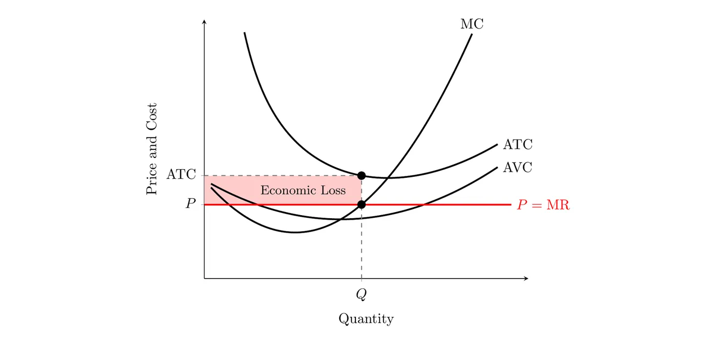
Economic loss: if price is below ATC at that quantity.

Shutdown decision: a losing firm keeps operating as long as price stays above AVC. If price drops below minimum AVC, shut down immediately to limit losses to just the fixed costs.

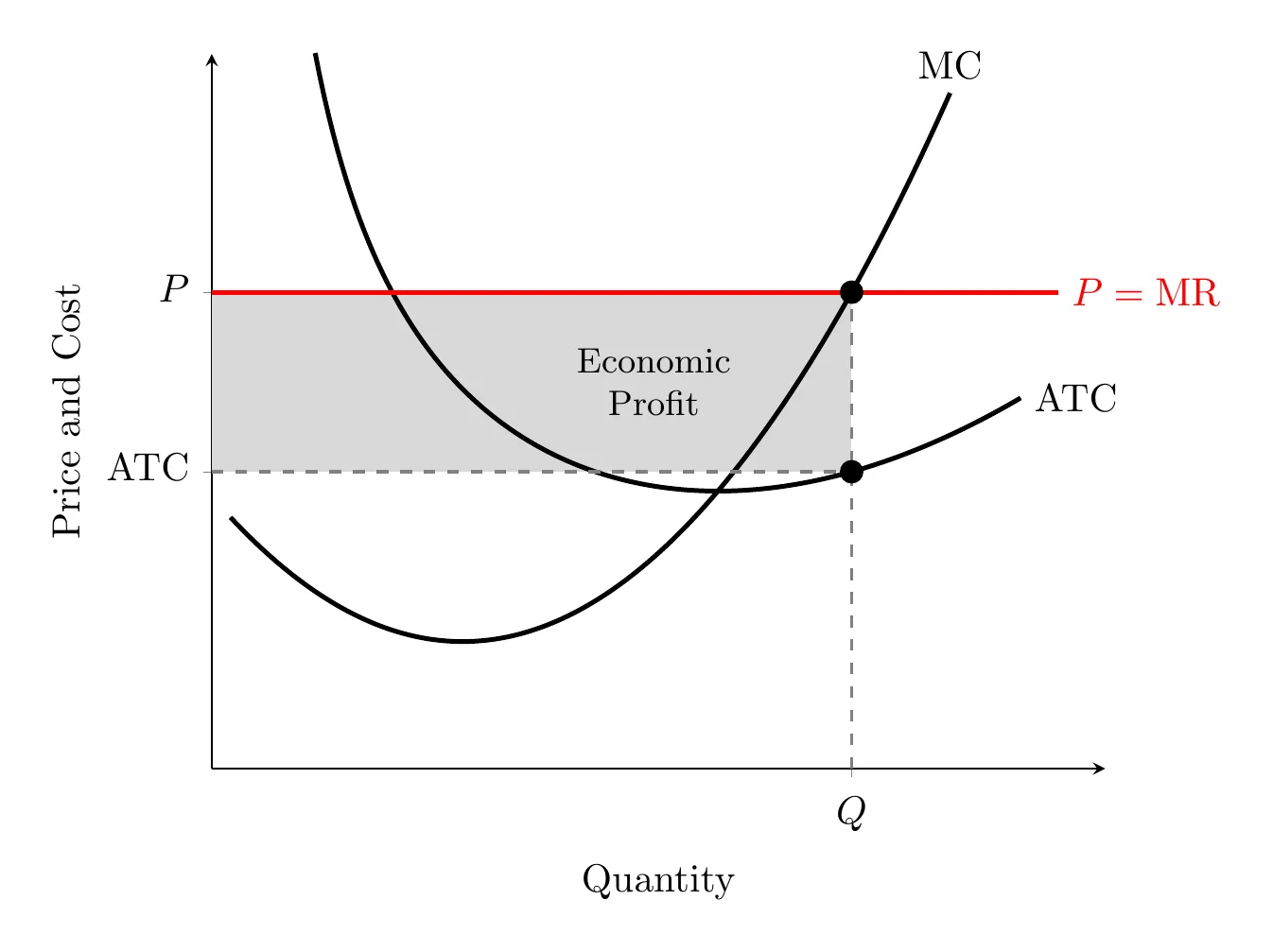
Calculating profit or loss: find the quantity where MR = MC, read ATC at that quantity, then:

\text{Profit} = (P - ATC) \times Q

Profit example: at P = $10, the profit-maximizing quantity is 5 units, and ATC there is $8. Profit = ($10 − $8) × 5 = $10. On the graph, that’s the shaded rectangle: its height is P − ATC and its width is Q.

Loss example: at P = $6, MR = MC at 4 units, and ATC there is $8.25. Profit = ($6 − $8.25) × 4 = −$9, a $9 loss. Price is still above AVC ($5.25), so the firm keeps producing in the short run.

When price is below ATC but above AVC, the same rectangle shows a loss instead:

Moving to Long-Run Equilibrium

Because entry barriers are low, short-run profits and losses don’t last.

From profit to break-even: new firms enter, supply shifts right, price falls until it hits the minimum of ATC.

From loss to break-even: firms exit, supply shifts left, price rises until survivors break even.

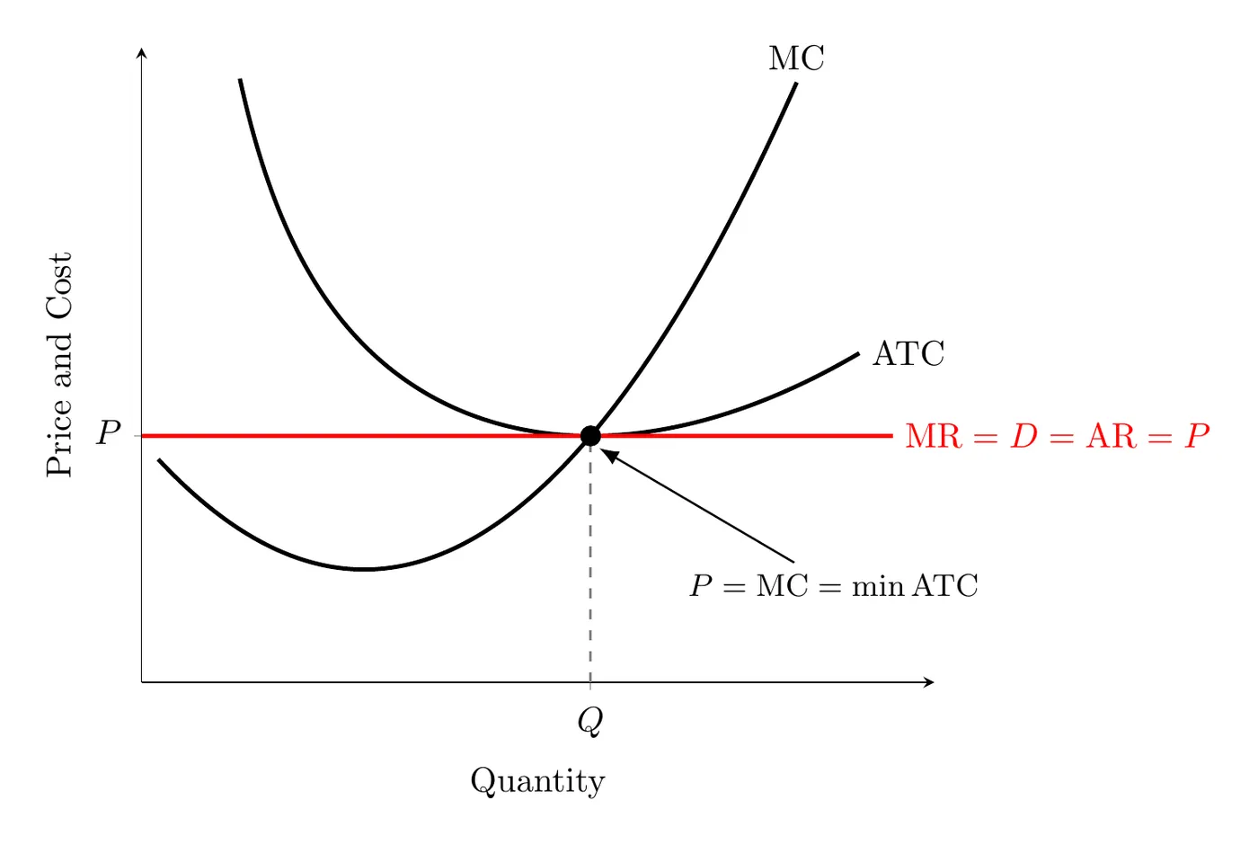
Long-run equilibrium: every firm earns zero economic profit (a normal profit), where $P = MC = \text{min } ATC$ .

Here’s the move from short-run profit to long-run equilibrium on side-by-side graphs:

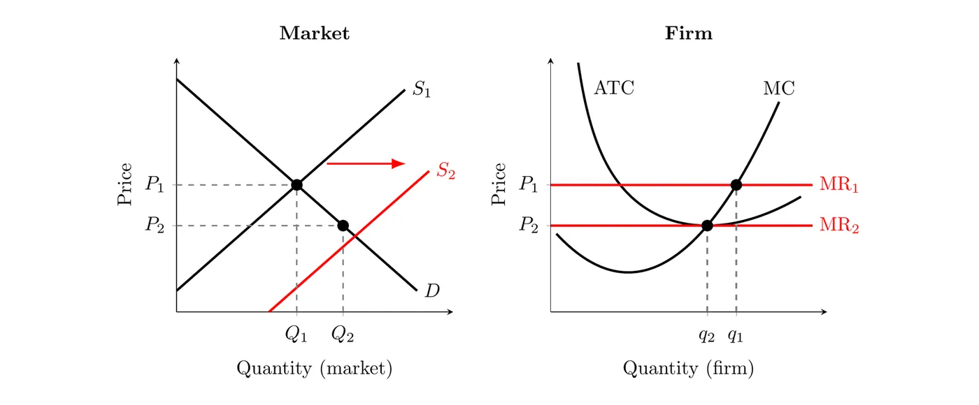
At $P_1$ , each firm produces $q_1$ (where $MR_1 = MC$ ) and earns an economic profit, since $P_1$ is above ATC.

The profit attracts new firms, so market supply shifts from $S_1$ to $S_2$ . The market price falls to $P_2$ and market quantity rises from $Q_1$ to $Q_2$ .

Each firm slides down its MC curve to $q_2$ , the bottom of ATC, where economic profit is zero. Each firm makes less ( $q_2 < q_1$ ), but there are more firms, so the market as a whole makes more.

A short-run loss works the same way in reverse: firms exit, supply shifts left, price rises back to the bottom of ATC, market quantity falls, and each surviving firm makes more.

Efficiency

Perfectly competitive firms are the gold standard for efficiency in the long run.

Allocative efficiency: producing the quantity society most wants, where $P = MC$ . Competitive firms always hit this, short run and long run alike.

At the market equilibrium, the price equals the buyer’s marginal benefit from the last unit bought (buyers keep buying until MB = P) and the seller’s marginal cost of the last unit made (firms keep producing until MC = P). So $MB = P = MC$ : every unit that’s worth more to buyers than it costs to make gets produced, and nothing beyond that.

Productive efficiency: producing at the lowest possible per-unit cost (minimum ATC). This only happens in the long run, once entry and exit force price down to the bottom of the ATC curve.

In long-run equilibrium, every firm still in the market produces at its efficient scale, the output at the bottom of its ATC curve. That’s why $P = MC = \text{min } ATC$ and economic profit is zero.

Both at once: in long-run equilibrium, a perfectly competitive market is both allocatively efficient ( $P = MC$ ) and productively efficient ( $P = \text{min } ATC$ ).

Prices as signals. In a competitive market, the price passes along information that no single buyer or seller has on their own, and gives everyone a reason to act on it:

For buyers: firms produce until MC = P, so the price tells buyers what it costs to make one more unit. A buyer only buys if that unit is worth at least the price to them.

For sellers: buyers keep buying until MB = P, so the price tells firms how much buyers value one more unit. A firm only makes that unit if it can do it for the price or less.

Example: a drought raises the cost of growing wheat. Supply falls and the price of wheat rises. Buyers who value wheat the least cut back, and farmers outside the drought area grow more. Nobody has to know about the drought: the higher price alone gets everyone to adjust, and the market still ends up where $P = MC$ .

Long-Run Cost Industries

How an industry responds to expansion depends on its cost structure:

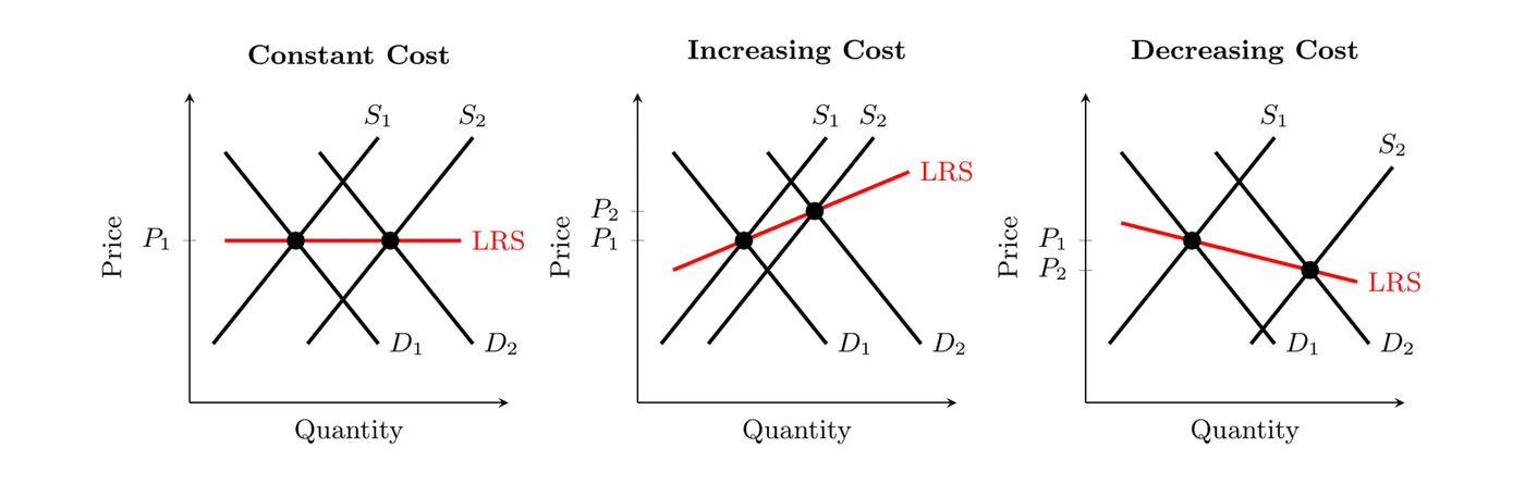
Constant cost industry: entry/exit doesn’t change resource costs. Long-run supply is perfectly elastic (horizontal).

If demand rises, entry continues until price falls all the way back to its old level, since every firm’s minimum ATC hasn’t changed. The long-run price stays the same; only quantity grows.

Increasing cost industry: as the industry grows, demand for resources drives their price up, shifting ATC up. Long-run supply slopes upward.

New firms bid up the prices of inputs (like specialized workers or land), so every firm’s ATC shifts up. The new long-run price is higher than before, at the new, higher minimum ATC.

Decreasing cost industry: expansion brings better infrastructure or cheaper resources (economies of scale), shifting ATC down. This creates a rare downward-sloping long-run supply curve.

Careful: this comes from the whole industry growing (like suppliers and trained workers clustering nearby), not from one firm getting bigger, so it’s different from a single firm’s economies of scale in 3.3. The new long-run price is lower than before, at the new, lower minimum ATC.

In every case, the long-run price ends up at the bottom of the firms’ ATC curves. What changes is where that bottom sits once the industry has grown. Connecting the old and new long-run equilibrium points traces out the long-run supply curve (LRS):

Bottom line: in a perfectly competitive market, firms are small, powerless price takers selling identical goods. They might see big profits or painful losses short term, but easy entry and exit always pull them back to zero economic profit in the long run, hitting both allocative and productive efficiency along the way.

Back Next