6.2 - Approximating Areas with Riemann Sums

Introduction

When a curve doesn’t form a nice geometric shape, we can’t use basic area formulas. Instead we approximate the area with rectangles or trapezoids.

To approximate area on

[a, b]

using

n

sub-intervals:

\boxed{\Delta x = \frac{b - a}{n}}

where

\Delta x

is the width of each sub-interval.

More sub-intervals means a better approximation.

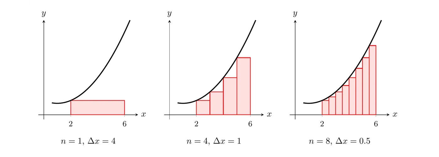
Riemann Sums

A Riemann sum approximates area by adding up the areas of multiple rectangles. It’s named after the German mathematician Bernhard Riemann.

For all four examples below, we’ll use the same function:

f(x) = 4x - \tfrac{1}{2}x^2 \quad \text{on } [2, 8], \quad n = 3

Width:

\Delta x = \frac{8 - 2}{3} = 2

Sub-intervals:

[2, 4]

[4, 6]

[6, 8]

Useful values:

f(2) = 6

f(4) = 8

f(6) = 6

f(8) = 0

Left Riemann Sum

Use the left endpoint of each sub-interval for the rectangle height.

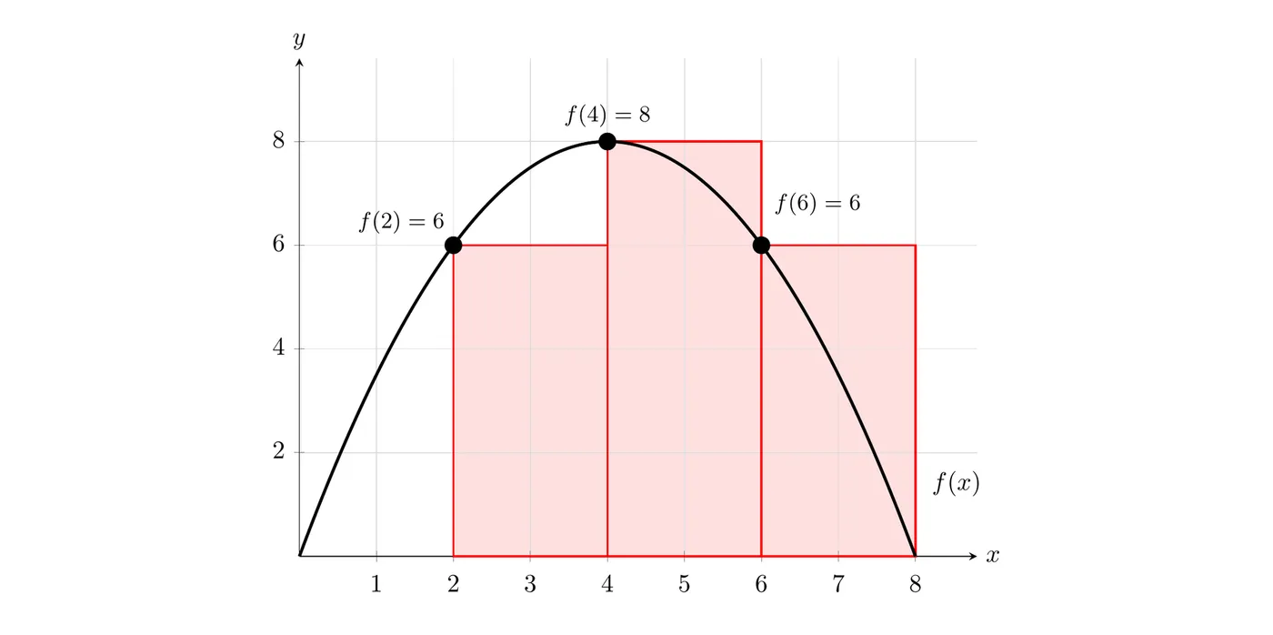
\text{Left Sum} = \Delta x [f(2) + f(4) + f(6)] = 2[6 + 8 + 6] = 2(20) = 40

The left Riemann sum approximation is 40 square units.

Right Riemann Sum

Use the right endpoint of each sub-interval for the height.

\text{Right Sum} = 2[f(4) + f(6) + f(8)] = 2[8 + 6 + 0] = 2(14) = 28

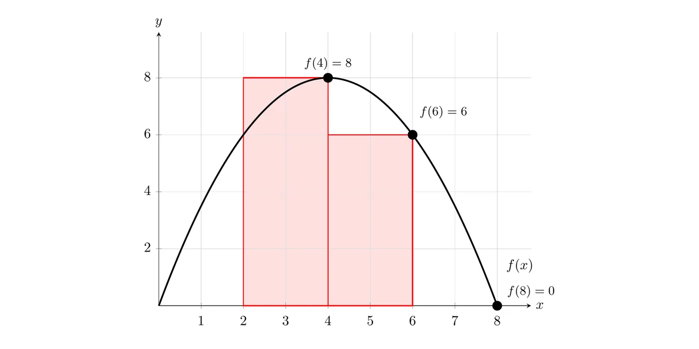
The right Riemann sum approximation is 28 square units. Note that

f(8) = 0

, so the third rectangle has zero height.

Midpoint Riemann Sum

Use the midpoint of each sub-interval for the height. The midpoints here are

3

5

, and

7

f(3) = 4(3) - \tfrac{1}{2}(9) = 12 - 4.5 = 7.5

f(5) = 4(5) - \tfrac{1}{2}(25) = 20 - 12.5 = 7.5

f(7) = 4(7) - \tfrac{1}{2}(49) = 28 - 24.5 = 3.5

\text{Midpoint Sum} = 2[7.5 + 7.5 + 3.5] = 2(18.5) = 37

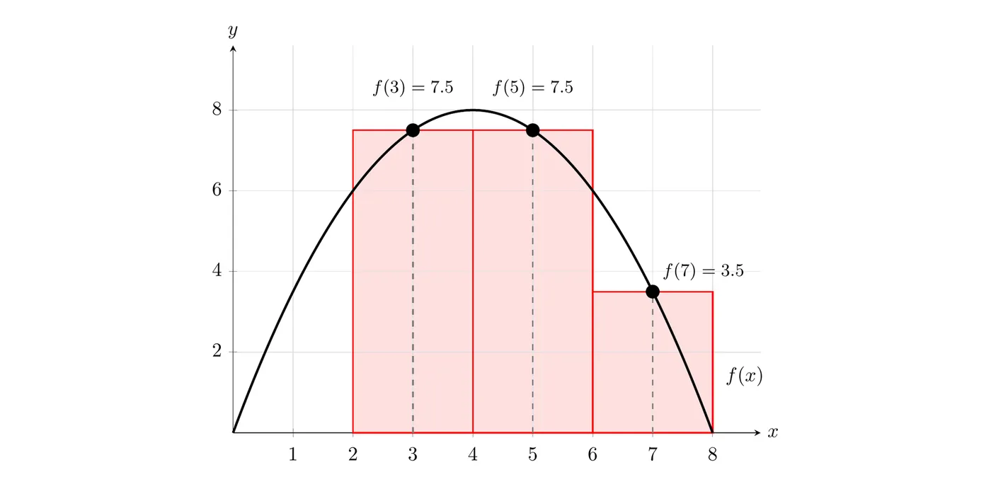
The midpoint approximation is 37 square units, which lands between the left sum (40) and the right sum (28).

Trapezoidal Sum

Use trapezoids instead of rectangles by connecting consecutive function values. A trapezoid has two different heights (the left and right endpoints).

\boxed{\text{Trapezoid area} = \Delta x \cdot \frac{f(x_{\text{left}}) + f(x_{\text{right}})}{2}}

That’s the width times the average of the two heights.

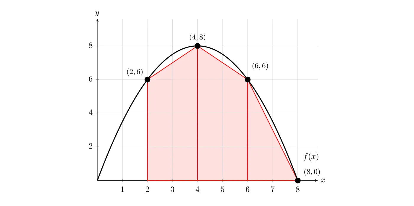
\text{Trap Sum} = 2\left[\frac{6 + 8}{2} + \frac{8 + 6}{2} + \frac{6 + 0}{2}\right] = 2[7 + 7 + 3] = 2(17) = 34

The trapezoidal approximation is 34 square units. The exact area is 36, so here the midpoint sum (37, off by 1) is actually closer than the trapezoidal sum (34, off by 2).

Over-estimates vs. Under-estimates

Whether a Riemann sum is over or under depends on two things: whether the function is increasing or decreasing, and which method you use.

For increasing functions

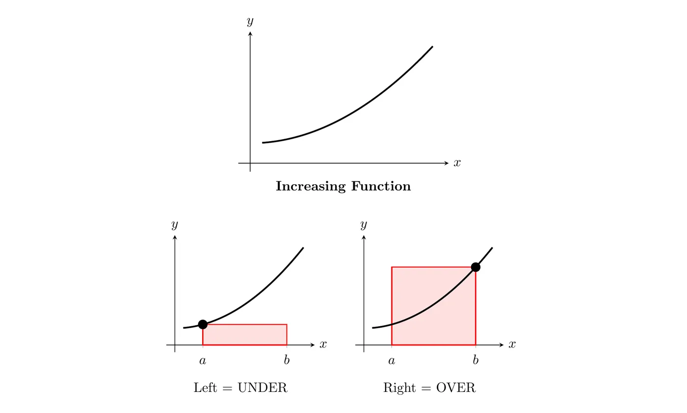
Method	Estimate Type
Left Riemann Sum	Under-estimate
Right Riemann Sum	Over-estimate

For decreasing functions

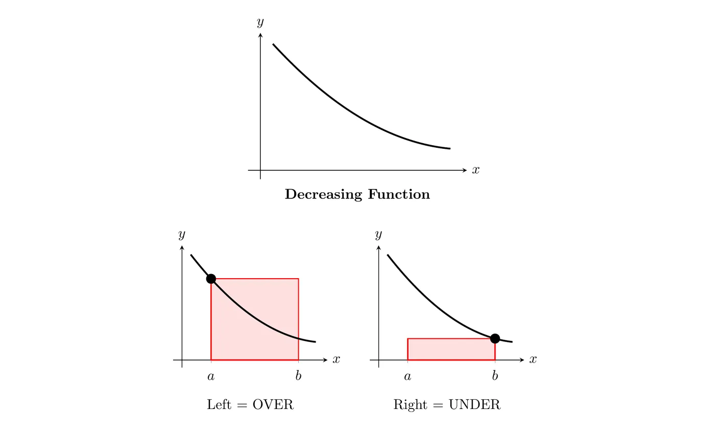
Method	Estimate Type
Left Riemann Sum	Over-estimate
Right Riemann Sum	Under-estimate

For trapezoidal sums, it depends on concavity.

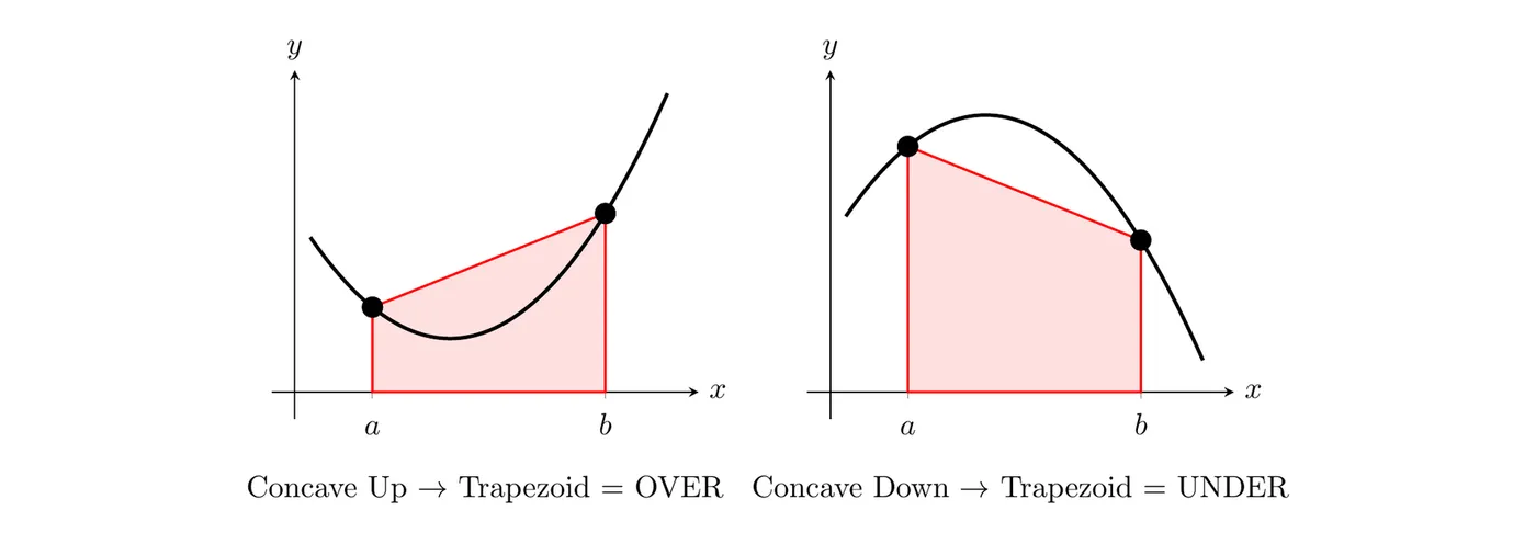
Concavity	Trapezoidal Estimate
Concave up	Over-estimate
Concave down	Under-estimate
Linear (no concavity)	Exact

For midpoint sums, it also depends on concavity, but the rule is the opposite of trapezoids.

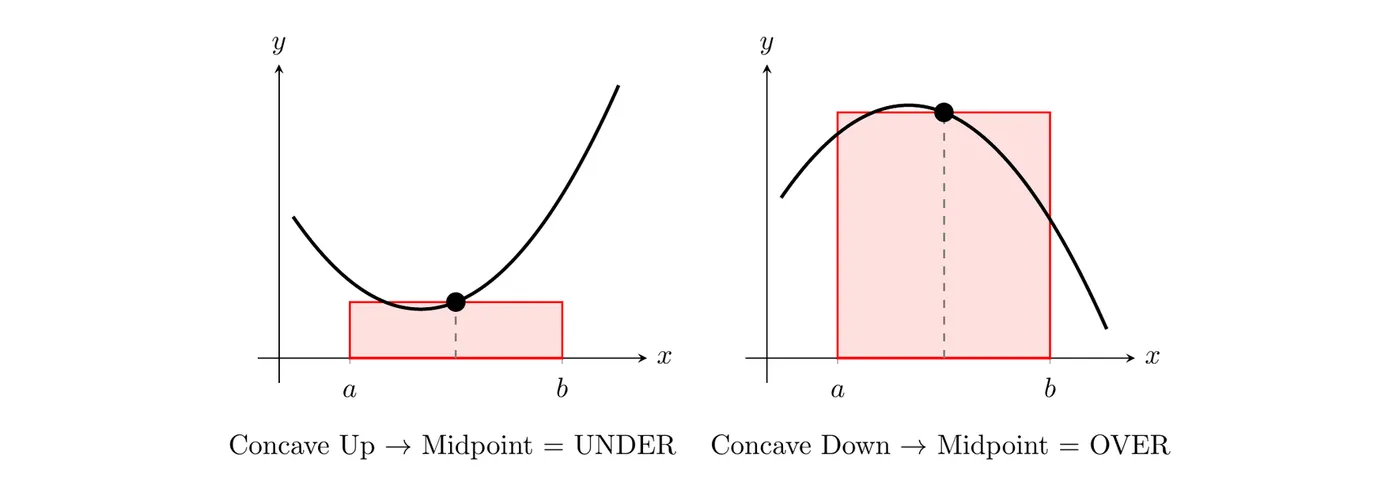
Concavity	Midpoint Estimate
Concave up	Under-estimate
Concave down	Over-estimate
Linear (no concavity)	Exact

Why? Tilt the top of a midpoint rectangle until it lines up with the tangent line at the midpoint. The area doesn’t change, because the small triangle you cut off on one side is the same size as the one you add on the other. A concave up curve sits above its tangent lines, so the rectangle comes out too small. Concave down is the reverse.

Check with the example above:

f(x) = 4x - \tfrac{1}{2}x^2

has

f''(x) = -1

, so it’s concave down. The midpoint sum (37) is over the exact area (36), and the trapezoidal sum (34) is under it, just like the tables say.

Memory aid: just sketch a quick picture to figure out over vs. under.

Riemann Sums with Tables of Values

When you’re given a table instead of an equation, use the table values directly.

Example: rate problem with a table

Water is pumped out of a tank at rate

R(t)

in gallons per minute. Approximate the total water pumped in 12 minutes.

$t$ (min)	0	3	6	9	12
$R(t)$ (gal/min)	7	13	18	23	27

Note that

R(t)

is increasing throughout.

Right Riemann sum (4 sub-intervals)

Sub-intervals

[0,3], [3,6], [6,9], [9,12]

, each with

\Delta t = 3

\text{Right Sum} = 3[13 + 18 + 23 + 27] = 3(81) = 243 \text{ gallons}

Justification: this is an over-estimate because it’s a right Riemann sum on an increasing function.

Left Riemann sum (4 sub-intervals)

\text{Left Sum} = 3[7 + 13 + 18 + 23] = 3(61) = 183 \text{ gallons}

Justification: this is an under-estimate because it’s a left Riemann sum on an increasing function.

Midpoint Riemann sum (2 sub-intervals)

Important: you can only use values that appear in the table, so you have to pick sub-intervals whose midpoints are actually there.

Sub-intervals

[0, 6]

and

[6, 12]

, each with

\Delta t = 6

. Midpoints are

t = 3

and

t = 9

, both in the table.

\text{Midpoint Sum} = 6[13 + 23] = 6(36) = 216 \text{ gallons}

You couldn’t use sub-intervals like

[0,3]

here, because the midpoint

t = 1.5

isn’t in the table.

Trapezoidal sum (4 sub-intervals)

\text{Trap Sum} = 3\left[\frac{7+13}{2} + \frac{13+18}{2} + \frac{18+23}{2} + \frac{23+27}{2}\right]

= 3[10 + 15.5 + 20.5 + 25] = 3(71) = 213 \text{ gallons}

Comparison

Method	Approximation	Type
Left Sum	183 gallons	Under
Right Sum	243 gallons	Over
Midpoint Sum	216 gallons	Between
Trapezoidal Sum	213 gallons	Between

General Formulas

Left Riemann sum

L_n = \Delta x [f(x_0) + f(x_1) + f(x_2) + \cdots + f(x_{n-1})]

Right Riemann sum

R_n = \Delta x [f(x_1) + f(x_2) + f(x_3) + \cdots + f(x_n)]

Midpoint Riemann sum

M_n = \Delta x [f(\bar{x}_1) + f(\bar{x}_2) + \cdots + f(\bar{x}_n)]

where

\bar{x}_i

is the midpoint of the

i

-th sub-interval.

Trapezoidal sum

T_n = \Delta x \left[\frac{f(x_0) + f(x_1)}{2} + \frac{f(x_1) + f(x_2)}{2} + \cdots + \frac{f(x_{n-1}) + f(x_n)}{2}\right]

Or in the compact form:

T_n = \frac{\Delta x}{2}[f(x_0) + 2f(x_1) + 2f(x_2) + \cdots + 2f(x_{n-1}) + f(x_n)]

Riemann Sums with Unequal Sub-intervals

Everything above used equal widths, but sub-intervals don’t have to be the same size, and tables on the AP exam often have uneven gaps. The rule doesn’t change: each rectangle or trapezoid uses its own width. You just can’t factor out one

\Delta x

, and the compact trapezoid formula above doesn’t apply.

Example: a hose fills a pool at a rate of

H(t)

gallons per minute, where

H

is increasing. Approximate the water that flows into the pool from

t = 0

t = 10

minutes.

$t$ (min)	0	2	5	6	10
$H(t)$ (gal/min)	12	15	20	21	25

The widths are 2, 3, 1, and 4 minutes.

Left Riemann sum

\text{Left Sum} = 2(12) + 3(15) + 1(20) + 4(21) = 24 + 45 + 20 + 84 = 173 \text{ gallons}

Right Riemann sum

\text{Right Sum} = 2(15) + 3(20) + 1(21) + 4(25) = 30 + 60 + 21 + 100 = 211 \text{ gallons}

Trapezoidal sum

\text{Trap Sum} = 2 \cdot \frac{12 + 15}{2} + 3 \cdot \frac{15 + 20}{2} + 1 \cdot \frac{20 + 21}{2} + 4 \cdot \frac{21 + 25}{2}

= 27 + 52.5 + 20.5 + 92 = 192 \text{ gallons}

Since

H

is increasing, the left sum is an under-estimate and the right sum is an over-estimate, so the actual amount is between 173 and 211 gallons.

Key Takeaways

Width formula: $\Delta x = \frac{b-a}{n}$ , where $n$ is the number of sub-intervals

More sub-intervals means a better approximation (and more work)

Left sum: left endpoint of each sub-interval for the height

Right sum: right endpoint for the height

Midpoint sum: midpoint for the height

Trapezoidal sum: average the two endpoint heights

Increasing function: left is under, right is over

Decreasing function: left is over, right is under

Trapezoids: concave up is over, concave down is under

Midpoints: concave up is under, concave down is over (the opposite of trapezoids)

Tables: you can only use the values given, so choose sub-intervals carefully for midpoints

Unequal widths: multiply each height by the width of its own sub-interval

Midpoint and trapezoidal sums are usually more accurate than left or right sums for the same number of sub-intervals

Justification: state both the method AND the function’s behavior (increasing/decreasing or concavity)

Units from a rate: the area gives the accumulation when you start with a rate of change

Back Next