6.3 - Riemann Sums, Summation Notation, and Definite Integral Notation

From Approximation to Exact Area

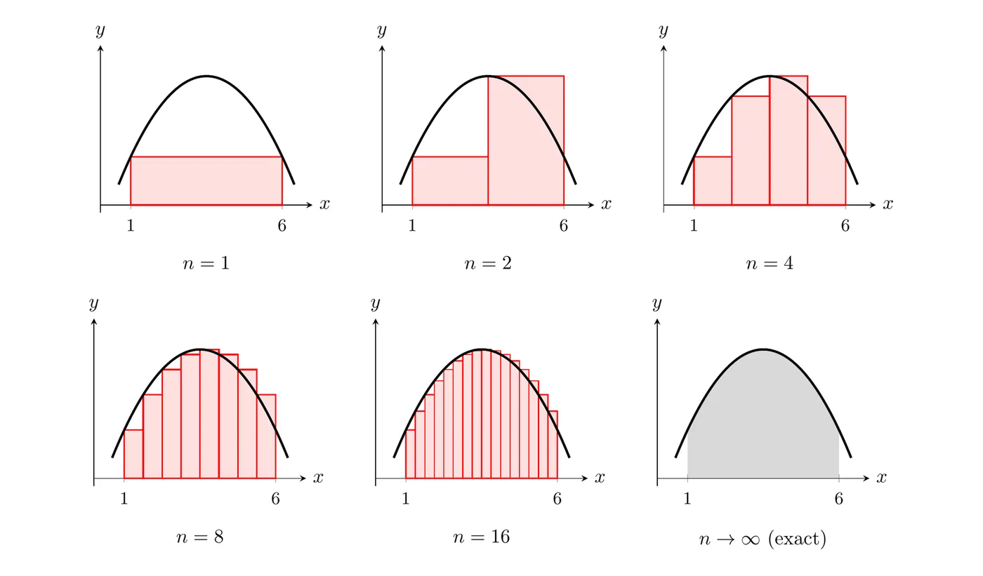
As the number of rectangles goes up, the approximation gets better. With infinitely many rectangles, we get the exact area.

6.3 - Riemann Sums, Summation Notation, and Definite Integral Notation

Width of Sub-intervals

For

[a, b]

divided into

n

sub-intervals:

\boxed{\Delta x = \frac{b - a}{n}}

n \to \infty

, the width

\Delta x \to 0

, meaning the rectangles become infinitesimally thin.

Summation Notation

The sum of all rectangle areas, written out:

\Delta x \cdot f(x_1) + \Delta x \cdot f(x_2) + \Delta x \cdot f(x_3) + \cdots + \Delta x \cdot f(x_n)

Each term is (width) × (height), the area of one rectangle. In summation notation:

\boxed{\sum_{k=1}^{n} \Delta x \cdot f(x_k)}

Reading it: -

\sum

means “sum of” -

k=1

means start at

k = 1

n

means end at

k = n

- Add up all the terms as

k

runs from 1 to

n

The Limit Definition of Area

To get the exact area, take the limit as the number of rectangles goes to infinity:

\boxed{\lim_{n \to \infty} \sum_{k=1}^{n} \Delta x \cdot f(x_k)}

Components: -

\Delta x = \frac{b-a}{n}

is the width of each rectangle -

f(x_k)

is the height of the

k

-th rectangle -

x_k = a + \frac{b-a}{n} \cdot k

is the

x

-position of the

k

-th rectangle

Putting it all together:

\lim_{n \to \infty} \sum_{k=1}^{n} \frac{b-a}{n} \cdot f\left(a + \frac{b-a}{n} \cdot k\right)

What’s happening: - Start at

x = a

- Add

k

widths, so

a + \Delta x \cdot k

gives the position of the

k

-th rectangle - Evaluate the function there for the height - Multiply width by height for each rectangle - Sum them all - Take the limit as

n \to \infty

Alternative notation

Instead of

n \to \infty

, you can write:

\lim_{\Delta x \to 0} \sum f(x_k) \Delta x

which emphasizes that the rectangle widths shrink to zero.

The Definite Integral

That summation notation is a mouthful. Calculus gives us something much cleaner:

\boxed{\int_a^b f(x) \, dx}

This means the exact area under the curve

f(x)

from

x = a

x = b

\int_a^b f(x) \, dx = \lim_{n \to \infty} \sum_{k=1}^{n} \frac{b-a}{n} \cdot f\left(a + \frac{b-a}{n} \cdot k\right)

Parts of the notation: -

\int

is the integral symbol (an elongated S, for “sum”) -

a

is the lower limit of integration -

b

is the upper limit of integration -

f(x)

is the function, called the integrand -

dx

says we’re integrating with respect to

x

The general definition

The formulas above use equal widths and right endpoints, because that version is the easiest to write. The official definition is more flexible:

Any widths: the sub-intervals don’t have to be the same size. The $i$ -th one has its own width $\Delta x_i$ .

Any point: the height can come from any point $x_i^*$ in the $i$ -th sub-interval (left endpoint, right endpoint, midpoint, or anywhere in between).

Sum of products: each term is the value of $f$ at that point times the width of that sub-interval.

\int_a^b f(x) \, dx = \lim_{\max \Delta x_i \to 0} \sum_{i=1}^{n} f(x_i^*) \, \Delta x_i

Taking the limit as the widest sub-interval shrinks to 0 forces every rectangle to get thin. For a continuous function, the limit is the same no matter which widths or points you use, so the right-endpoint version with

x_k = a + \frac{b-a}{n} \cdot k

works fine. (Left endpoints would use

a + \frac{b-a}{n} \cdot (k - 1)

instead.)

f

is negative on part of the interval, those products

f(x_i^*) \, \Delta x_i

are negative. That’s why area below the x-axis counts as negative in a definite integral.

Converting: Integral to Summation

Example 1:

\displaystyle \int_3^7 (2x + 5) \, dx

\lim_{n \to \infty} \sum_{k=1}^{n} \frac{7-3}{n} \cdot \left[2\left(3 + \frac{7-3}{n} \cdot k\right) + 5\right]

Step by step: 1.

a = 3

b = 7

2. Width:

\Delta x = \frac{7-3}{n} = \frac{4}{n}

3. Position:

x_k = 3 + \frac{4}{n} \cdot k

4. Function:

f(x) = 2x + 5

5. Substitute:

f(x_k) = 2\left(3 + \frac{4}{n}k\right) + 5

Simplified:

\lim_{n \to \infty} \sum_{k=1}^{n} \frac{4}{n} \left[6 + \frac{8k}{n} + 5\right] = \lim_{n \to \infty} \sum_{k=1}^{n} \frac{4}{n} \left[11 + \frac{8k}{n}\right]

Example 2:

\displaystyle \int_1^5 x^2 \, dx

\lim_{n \to \infty} \sum_{k=1}^{n} \frac{4}{n} \left[1 + \frac{4k}{n}\right]^2

Breakdown: - Interval

[1, 5]

, so

b - a = 4

- Width:

\frac{4}{n}

x_k = 1 + \frac{4k}{n}

f(x_k) = \left(1 + \frac{4k}{n}\right)^2

Converting: Summation to Integral

One summation can correspond to multiple integral forms, depending on where you decide the interval starts.

Given:

\displaystyle \lim_{n \to \infty} \sum_{k=1}^{n} \frac{6}{n} \left(4 + \frac{6k}{n}\right)^2

These three integrals are all equal to that same limit:

\int_0^6 (4 + x)^2 \, dx \quad = \quad \int_4^{10} x^2 \, dx \quad = \quad \int_0^1 6(4+6x)^2 \, dx

Form 1:

\displaystyle \int_0^6 (4 + x)^2 \, dx

- Width

\frac{6}{n}

means

b - a = 6

- Starting at

a = 0

x_k = \frac{6k}{n}

- Function:

(4 + x)^2

Form 2:

\displaystyle \int_4^{10} x^2 \, dx

- Width

\frac{6}{n}

means

b - a = 6

- Starting at

a = 4

x_k = 4 + \frac{6k}{n}

- That’s exactly the expression being squared, so the function is just

x^2

Form 3:

\displaystyle \int_0^1 6(4 + 6x)^2 \, dx

- Rewrite

\frac{6}{n} = 6 \cdot \frac{1}{n}

, so the width is

\frac{1}{n}

and

b - a = 1

- Starting at

a = 0

x_k = \frac{k}{n}

- The factored-out 6 becomes part of the function

Converting: Series to Integral

Example: a written-out sum

\frac{2}{n} \left[3 + \frac{2 \cdot 1}{n}\right] + \frac{2}{n}\left[3 + \frac{2 \cdot 2}{n}\right] + \cdots + \frac{2}{n}\left[3 + \frac{2 \cdot n}{n}\right]

Identify the components: - Width:

\Delta x = \frac{2}{n}

, so

b - a = 2

- With

a = 0

, that gives

b = 2

- The changing part is

3 + \frac{2k}{n}

, where the 3 is a constant shift -

\frac{2k}{n}

is playing the role of

x

, running from 0 to 2

Since

x_k = \frac{2k}{n}

, the expression

3 + \frac{2k}{n}

is just

3 + x

, so

f(x) = x + 3

\int_0^2 (x + 3) \, dx

Example: with a trig function

\frac{1}{10}\left[\cos\left(\frac{1}{10}\right) + \cos\left(\frac{2}{10}\right) + \cos\left(\frac{3}{10}\right) + \cdots + \cos\left(\frac{10}{10}\right)\right]

Analysis: - Width

\frac{1}{10}

, so with

n = 10

we get

b - a = 1

- The arguments are

\frac{k}{10}

for

k = 1

through

10

- Those run from

\frac{1}{10}

up to

\frac{10}{10} = 1

- Starting point

a = 0

, ending point

b = 1

\int_0^1 \cos(x) \, dx

Key insight: the 10 here represents

n

, the number of sub-intervals. It isn’t part of the integral. Any

n

would give the same integral.

Careful with the limit. A sum with a fixed number of terms, like this one with

n = 10

, is a right Riemann sum, so it only approximates

\int_0^1 \cos(x) \, dx

. (The sum is about 0.818, and the integral is about 0.841.) A Riemann sum equals the integral exactly only in the limit as

n \to \infty

, so an expression that equals a definite integral has

\lim_{n \to \infty}

in front of the sum. The same goes for the written-out sum in the first example.

Example: polynomial

\frac{5}{n}\sum_{k=1}^{n}\left[\left(\frac{5k}{n}\right)^3 - 2\right]

Width: $\frac{5}{n}$ , so $b - a = 5$

Starting at $a = 0$ : $x_k = \frac{5k}{n}$

Function: $x^3 - 2$

\int_0^5 (x^3 - 2) \, dx

Strategy for Conversions

Summation → integral

Identify $\Delta x$ : look for the $\frac{b-a}{n}$ width term

Determine the interval: if you’re given the starting point, get $b - a$ from the width; otherwise pull it from the expression

Find $x_k$ : look for the pattern $a + \frac{b-a}{n} \cdot k$

Extract the function: whatever $x_k$ is being plugged into becomes $f(x)$

Integral → summation

Identify $a$ and $b$

Calculate the width: $\Delta x = \frac{b-a}{n}$

Write $x_k$ : $x_k = a + \frac{b-a}{n} \cdot k$

Substitute into the function: replace $x$ with $x_k$

Build the sum: $\displaystyle \lim_{n \to \infty} \sum_{k=1}^{n} \Delta x \cdot f(x_k)$

Common Patterns

Summation Element	Meaning
$\frac{c}{n}$	Width of rectangles, where $c = b - a$
$a + \frac{b-a}{n} \cdot k$	Position of the $k$ -th rectangle
$\sum_{k=1}^{n}$	Sum from the 1st to the $n$ -th rectangle
$\lim_{n \to \infty}$	Take infinitely many rectangles

Key Takeaways

More rectangles means a better approximation. As $n \to \infty$ , the approximation becomes the exact area

Width formula: $\Delta x = \frac{b-a}{n}$ , and as $n \to \infty$ , $\Delta x \to 0$

Summation notation: $\displaystyle \sum_{k=1}^{n} (\text{width}) \times (\text{height})$

Position formula: $x_k = a + \frac{b-a}{n} \cdot k$ , which tells you where to evaluate the height

Limit of a Riemann sum: $\displaystyle \lim_{n \to \infty} \sum_{k=1}^{n} \frac{b-a}{n} \cdot f\left(a + \frac{b-a}{n} \cdot k\right)$

Definite integral notation: $\displaystyle \int_a^b f(x) \, dx$ is the exact area under the curve

Equivalence: the definite integral IS the limit of a Riemann sum

Multiple forms possible: one integral can have several summation representations

The $n$ in summations is the number of rectangles, not part of the integral

On exams: these conversions usually show up as multiple choice, so test each option

Foundation concept: integrals are the basis for everything in integral calculus

Back Next