Introduction to Antiderivatives An
antiderivative of a function
f f f is a function
F F F whose derivative is
f f f .
If F ′ ( x ) = f ( x ) , then F ( x ) is an antiderivative of f ( x ) \text{If } F'(x) = f(x), \text{ then } F(x) \text{ is an antiderivative of } f(x) If F ′ ( x ) = f ( x ) , then F ( x ) is an antiderivative of f ( x ) Example If
F ( x ) = 3 x 2 F(x) = 3x^2 F ( x ) = 3 x 2 , then
F ′ ( x ) = 6 x F'(x) = 6x F ′ ( x ) = 6 x .
So
3 x 2 3x^2 3 x 2 is an
antiderivative of
6 x 6x 6 x .
Verification: take the derivative to check.
d d x [ 3 x 2 ] = 6 x ✓ \frac{d}{dx}[3x^2] = 6x \,\checkmark d x d [ 3 x 2 ] = 6 x ✓ Connection to Integrals Key insight: the change in an antiderivative,
F ( b ) − F ( a ) F(b)-F(a) F ( b ) − F ( a ) , gives the net
area under the curve .
When we evaluate
∫ a b f ( x ) d x \int_a^b f(x) \, dx ∫ a b f ( x ) d x , we’re finding the antiderivative
F ( x ) F(x) F ( x ) and using it to calculate the area.
This connection wasn’t obvious even to Newton and Leibniz.
Power Rule for Antiderivatives Review: Power Rule for Derivatives d d x [ x n ] = n x n − 1 \frac{d}{dx}[x^n] = nx^{n-1} d x d [ x n ] = n x n − 1 Steps:
Multiply by the exponent Subtract 1 from the exponent Power Rule for Antiderivatives (the Reverse Process) ∫ x n d x = x n + 1 n + 1 + C ( n ≠ − 1 ) \boxed{\int x^n \, dx = \frac{x^{n+1}}{n+1} + C \quad (n \neq -1)} ∫ x n d x = n + 1 x n + 1 + C ( n = − 1 ) Steps:
Add 1 to the exponentDivide by the new exponentAdd the constant C C C The Constant of Integration When finding antiderivatives, you have to include
+ C +C + C , where
C C C is an arbitrary constant.
Why? Because the derivative of any constant is zero:
d d x [ 3 x 2 + 5 ] = 6 x \frac{d}{dx}[3x^2 + 5] = 6x d x d [ 3 x 2 + 5 ] = 6 x d d x [ 3 x 2 − 17 ] = 6 x \frac{d}{dx}[3x^2 - 17] = 6x d x d [ 3 x 2 − 17 ] = 6 x d d x [ 3 x 2 + C ] = 6 x \frac{d}{dx}[3x^2 + C] = 6x d x d [ 3 x 2 + C ] = 6 x All of these functions have the same derivative, so they’re all antiderivatives of
6 x 6x 6 x .
Examples: Finding Antiderivatives Example 1: Basic Polynomial Find
∫ x 2 d x \int x^2 \, dx ∫ x 2 d x .
∫ x 2 d x = x 2 + 1 2 + 1 + C = x 3 3 + C \int x^2 \, dx = \frac{x^{2+1}}{2+1} + C = \frac{x^3}{3} + C ∫ x 2 d x = 2 + 1 x 2 + 1 + C = 3 x 3 + C Check: d d x [ x 3 3 + C ] = 3 x 2 3 = x 2 ✓ \frac{d}{dx}\left[\frac{x^3}{3} + C\right] = \frac{3x^2}{3} = x^2 \,\checkmark d x d [ 3 x 3 + C ] = 3 3 x 2 = x 2 ✓ Example 2: Multiple Terms Find
∫ ( 5 x 3 + 6 x − 3 − 1 ) d x \int \left(5x^3 + 6x^{-3} - 1\right) dx ∫ ( 5 x 3 + 6 x − 3 − 1 ) d x .
Step 1: Rewrite for clarity.
∫ ( 5 x 3 + 6 x − 3 − 1 ) d x \int \left(5x^3 + 6x^{-3} - 1\right) dx ∫ ( 5 x 3 + 6 x − 3 − 1 ) d x Step 2: Apply the power rule to each term.
= 5 ⋅ x 3 + 1 3 + 1 + 6 ⋅ x − 3 + 1 − 3 + 1 − x + C = 5 \cdot \frac{x^{3+1}}{3+1} + 6 \cdot \frac{x^{-3+1}}{-3+1} - x + C = 5 ⋅ 3 + 1 x 3 + 1 + 6 ⋅ − 3 + 1 x − 3 + 1 − x + C = 5 ⋅ x 4 4 + 6 ⋅ x − 2 − 2 − x + C = 5 \cdot \frac{x^4}{4} + 6 \cdot \frac{x^{-2}}{-2} - x + C = 5 ⋅ 4 x 4 + 6 ⋅ − 2 x − 2 − x + C = 5 x 4 4 − 6 2 x 2 − x + C = \frac{5x^4}{4} - \frac{6}{2x^2} - x + C = 4 5 x 4 − 2 x 2 6 − x + C = 5 x 4 4 − 3 x 2 − x + C = \frac{5x^4}{4} - \frac{3}{x^2} - x + C = 4 5 x 4 − x 2 3 − x + C Example 3: Radicals and Fractions Find
∫ ( x 1 / 2 + 3 x − 1 / 2 ) d x \int \left(x^{1/2} + 3x^{-1/2}\right) dx ∫ ( x 1/2 + 3 x − 1/2 ) d x .
= x 1 / 2 + 1 1 / 2 + 1 + 3 ⋅ x − 1 / 2 + 1 − 1 / 2 + 1 + C = \frac{x^{1/2+1}}{1/2+1} + 3 \cdot \frac{x^{-1/2+1}}{-1/2+1} + C = 1/2 + 1 x 1/2 + 1 + 3 ⋅ − 1/2 + 1 x − 1/2 + 1 + C = x 3 / 2 3 / 2 + 3 ⋅ x 1 / 2 1 / 2 + C = \frac{x^{3/2}}{3/2} + 3 \cdot \frac{x^{1/2}}{1/2} + C = 3/2 x 3/2 + 3 ⋅ 1/2 x 1/2 + C Simplify by multiplying by the reciprocals:
= 2 3 x 3 / 2 + 6 x 1 / 2 + C = 2 3 x 3 / 2 + 6 x + C = \frac{2}{3}x^{3/2} + 6x^{1/2} + C = \frac{2}{3}x^{3/2} + 6\sqrt{x} + C = 3 2 x 3/2 + 6 x 1/2 + C = 3 2 x 3/2 + 6 x + C Antiderivatives of Trigonometric Functions Sine and Cosine Derivative relationships:
d d x [ sin x ] = cos x ⇒ ∫ cos x d x = sin x + C \frac{d}{dx}[\sin x] = \cos x \quad \Rightarrow \quad \boxed{\int \cos x \, dx = \sin x + C} d x d [ sin x ] = cos x ⇒ ∫ cos x d x = sin x + C d d x [ cos x ] = − sin x ⇒ ∫ sin x d x = − cos x + C \frac{d}{dx}[\cos x] = -\sin x \quad \Rightarrow \quad \boxed{\int \sin x \, dx = -\cos x + C} d x d [ cos x ] = − sin x ⇒ ∫ sin x d x = − cos x + C Memory aid: work backwards from the derivatives.
Check for sine:
d d x [ − cos x + C ] = − ( − sin x ) = sin x ✓ \frac{d}{dx}[-\cos x + C] = -(-\sin x) = \sin x \,\checkmark d x d [ − cos x + C ] = − ( − sin x ) = sin x ✓ The Fundamental Theorem of Calculus (Part 1) Statement: if
f f f is continuous on
[ a , b ] [a, b] [ a , b ] , then
∫ a b f ( x ) d x = F ( b ) − F ( a ) \boxed{\int_a^b f(x) \, dx = F(b) - F(a)} ∫ a b f ( x ) d x = F ( b ) − F ( a ) where
F F F is any antiderivative of
f f f (meaning
F ′ ( x ) = f ( x ) F'(x) = f(x) F ′ ( x ) = f ( x ) ).
In words:
Find an antiderivative F ( x ) F(x) F ( x ) f ( x ) f(x) f ( x ) Evaluate F F F F ( b ) F(b) F ( b ) Evaluate F F F F ( a ) F(a) F ( a ) Subtract: F ( b ) − F ( a ) F(b) - F(a) F ( b ) − F ( a ) Notation ∫ a b f ( x ) d x = F ( x ) ∣ a b \int_a^b f(x) \, dx = F(x) \Big|_a^b ∫ a b f ( x ) d x = F ( x ) a b The vertical bar notation reminds you to evaluate at both limits.
Why + C +C + C When you evaluate a definite integral:
[ F ( b ) + C ] − [ F ( a ) + C ] = F ( b ) − F ( a ) [F(b) + C] - [F(a) + C] = F(b) - F(a) [ F ( b ) + C ] − [ F ( a ) + C ] = F ( b ) − F ( a ) The constants cancel, so you don’t need to write
+ C +C + C for definite integrals.
Why the Theorem Works Topic 6.4 showed that when
f f f is continuous,
A ( x ) = ∫ a x f ( t ) d t A(x) = \int_a^x f(t) \, dt A ( x ) = ∫ a x f ( t ) d t is an antiderivative of
f f f , because
A ′ ( x ) = f ( x ) A'(x) = f(x) A ′ ( x ) = f ( x ) . Any other antiderivative
F F F differs from
A A A by a constant, so
F ( x ) = A ( x ) + C F(x) = A(x) + C F ( x ) = A ( x ) + C . Then
F ( b ) − F ( a ) = [ A ( b ) + C ] − [ A ( a ) + C ] = A ( b ) − A ( a ) = ∫ a b f ( t ) d t − 0 F(b) - F(a) = [A(b) + C] - [A(a) + C] = A(b) - A(a) = \int_a^b f(t) \, dt - 0 F ( b ) − F ( a ) = [ A ( b ) + C ] − [ A ( a ) + C ] = A ( b ) − A ( a ) = ∫ a b f ( t ) d t − 0 since
A ( a ) = ∫ a a f ( t ) d t = 0 A(a) = \int_a^a f(t) \, dt = 0 A ( a ) = ∫ a a f ( t ) d t = 0 . That’s why
any antiderivative works.
Evaluating Definite Integrals Example 1: Linear Function Evaluate
∫ − 2 5 ( 4 − 6 x ) d x \int_{-2}^5 (4 - 6x) \, dx ∫ − 2 5 ( 4 − 6 x ) d x .
Step 1: Find the antiderivative.
F ( x ) = 4 x − 6 x 2 2 = 4 x − 3 x 2 F(x) = 4x - \frac{6x^2}{2} = 4x - 3x^2 F ( x ) = 4 x − 2 6 x 2 = 4 x − 3 x 2 Step 2: Evaluate at the bounds.
= [ 4 x − 3 x 2 ] − 2 5 = \left[4x - 3x^2\right]_{-2}^5 = [ 4 x − 3 x 2 ] − 2 5 = [ 4 ( 5 ) − 3 ( 5 ) 2 ] − [ 4 ( − 2 ) − 3 ( − 2 ) 2 ] = [4(5) - 3(5)^2] - [4(-2) - 3(-2)^2] = [ 4 ( 5 ) − 3 ( 5 ) 2 ] − [ 4 ( − 2 ) − 3 ( − 2 ) 2 ] = [ 20 − 75 ] − [ − 8 − 12 ] = [20 - 75] - [-8 - 12] = [ 20 − 75 ] − [ − 8 − 12 ] = − 55 − ( − 20 ) = − 55 + 20 = − 35 = -55 - (-20) = -55 + 20 = -35 = − 55 − ( − 20 ) = − 55 + 20 = − 35 Step 3: Check with a calculator.
On a TI-84:
MATH →
9:fnInt(4-6x, x, -2, 5) gives
− 35 -35 − 35 .
✓ \checkmark ✓ Example 2: With Radicals Evaluate
∫ 1 4 ( x − 1 x 2 ) d x \int_1^4 \left(\sqrt{x} - \dfrac{1}{x^2}\right) dx ∫ 1 4 ( x − x 2 1 ) d x .
Step 1: Rewrite with exponents.
∫ 1 4 ( x 1 / 2 − x − 2 ) d x \int_1^4 \left(x^{1/2} - x^{-2}\right) dx ∫ 1 4 ( x 1/2 − x − 2 ) d x Step 2: Find the antiderivative.
= [ x 3 / 2 3 / 2 − x − 1 − 1 ] 1 4 = [ 2 3 x 3 / 2 + 1 x ] 1 4 = \left[\frac{x^{3/2}}{3/2} - \frac{x^{-1}}{-1}\right]_1^4 = \left[\frac{2}{3}x^{3/2} + \frac{1}{x}\right]_1^4 = [ 3/2 x 3/2 − − 1 x − 1 ] 1 4 = [ 3 2 x 3/2 + x 1 ] 1 4 Step 3: Evaluate at the bounds.
Upper limit (
x = 4 x = 4 x = 4 ):
2 3 ( 4 ) 3 / 2 + 1 4 = 2 3 ( 4 ) 3 + 1 4 = 2 3 ( 8 ) + 1 4 = 16 3 + 1 4 \frac{2}{3}(4)^{3/2} + \frac{1}{4} = \frac{2}{3}(\sqrt{4})^3 + \frac{1}{4} = \frac{2}{3}(8) + \frac{1}{4} = \frac{16}{3} + \frac{1}{4} 3 2 ( 4 ) 3/2 + 4 1 = 3 2 ( 4 ) 3 + 4 1 = 3 2 ( 8 ) + 4 1 = 3 16 + 4 1 Lower limit (
x = 1 x = 1 x = 1 ):
2 3 ( 1 ) 3 / 2 + 1 1 = 2 3 + 1 = 5 3 \frac{2}{3}(1)^{3/2} + \frac{1}{1} = \frac{2}{3} + 1 = \frac{5}{3} 3 2 ( 1 ) 3/2 + 1 1 = 3 2 + 1 = 3 5 Subtract:
= 16 3 + 1 4 − 5 3 = 11 3 + 1 4 = \frac{16}{3} + \frac{1}{4} - \frac{5}{3} = \frac{11}{3} + \frac{1}{4} = 3 16 + 4 1 − 3 5 = 3 11 + 4 1 Convert to a common denominator of 12:
= 44 12 + 3 12 = 47 12 = \frac{44}{12} + \frac{3}{12} = \frac{47}{12} = 12 44 + 12 3 = 12 47 Check: a calculator gives about
3.9167 3.9167 3.9167 , which is
47 ÷ 12 47 \div 12 47 ÷ 12 .
✓ \checkmark ✓ Example 3: With a Constant Factor Evaluate
∫ − 1 2 4 sin ( x ) d x \int_{-1}^2 4\sin(x) \, dx ∫ − 1 2 4 sin ( x ) d x .
Factor out the constant:
= 4 ∫ − 1 2 sin ( x ) d x = 4 [ − cos ( x ) ] − 1 2 = 4\int_{-1}^2 \sin(x) \, dx = 4\left[-\cos(x)\right]_{-1}^2 = 4 ∫ − 1 2 sin ( x ) d x = 4 [ − cos ( x ) ] − 1 2 = 4 [ ( − cos ( 2 ) ) − ( − cos ( − 1 ) ) ] = 4 [ − cos ( 2 ) + cos ( 1 ) ] = 4[(-\cos(2)) - (-\cos(-1))] = 4[-\cos(2) + \cos(1)] = 4 [( − cos ( 2 )) − ( − cos ( − 1 ))] = 4 [ − cos ( 2 ) + cos ( 1 )] Evaluate numerically with a calculator: about
3.826 3.826 3.826 .
Application: Finding a Function from Its Derivative Problem type: you’re given
f ′ ( x ) f'(x) f ′ ( x ) and one point on
f ( x ) f(x) f ( x ) , and you need
f ( x ) f(x) f ( x ) at another point.
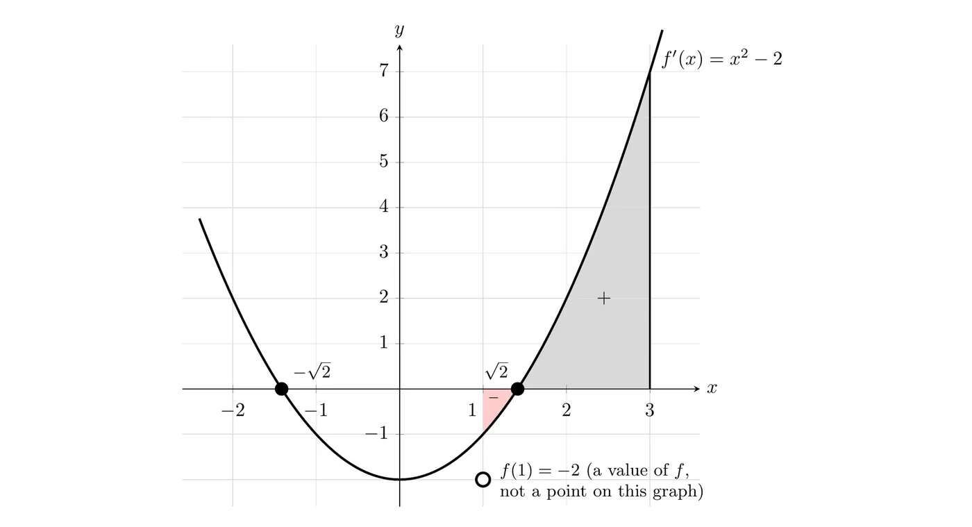
Example: Accumulation from a Rate Given:
f ′ ( x ) = x 2 − 2 f'(x) = x^2 - 2 f ′ ( x ) = x 2 − 2 f ( 1 ) = − 2 f(1) = -2 f ( 1 ) = − 2 Solution strategy:
f ( 3 ) = f ( 1 ) + ∫ 1 3 f ′ ( x ) d x f(3) = f(1) + \int_1^3 f'(x) \, dx f ( 3 ) = f ( 1 ) + ∫ 1 3 f ′ ( x ) d x In other words, final value = initial value + accumulated change .
Calculate:
f ( 3 ) = − 2 + ∫ 1 3 ( x 2 − 2 ) d x f(3) = -2 + \int_1^3 (x^2 - 2) \, dx f ( 3 ) = − 2 + ∫ 1 3 ( x 2 − 2 ) d x = − 2 + [ x 3 3 − 2 x ] 1 3 = -2 + \left[\frac{x^3}{3} - 2x\right]_1^3 = − 2 + [ 3 x 3 − 2 x ] 1 3 Upper limit (
x = 3 x = 3 x = 3 ):
27 3 − 6 = 9 − 6 = 3 \frac{27}{3} - 6 = 9 - 6 = 3 3 27 − 6 = 9 − 6 = 3 Lower limit (
x = 1 x = 1 x = 1 ):
1 3 − 2 = − 5 3 \frac{1}{3} - 2 = -\frac{5}{3} 3 1 − 2 = − 3 5 Difference:
3 − ( − 5 3 ) = 3 + 5 3 = 14 3 3 - \left(-\frac{5}{3}\right) = 3 + \frac{5}{3} = \frac{14}{3} 3 − ( − 3 5 ) = 3 + 3 5 = 3 14 So
f ( 3 ) = − 2 + 14 3 = − 6 + 14 3 = 8 3 f(3) = -2 + \frac{14}{3} = \frac{-6 + 14}{3} = \frac{8}{3} f ( 3 ) = − 2 + 3 14 = 3 − 6 + 14 = 3 8 Answer: f ( 3 ) = 8 3 = 2 2 3 f(3) = \dfrac{8}{3} = 2\frac{2}{3} f ( 3 ) = 3 8 = 2 3 2 Interpretation: starting at
f ( 1 ) = − 2 f(1) = -2 f ( 1 ) = − 2 , we accumulate the area under
f ′ ( x ) f'(x) f ′ ( x ) from 1 to 3, and that area is the net change in
f f f .
Key Takeaways Antiderivative: a function F F F F ′ ( x ) = f ( x ) F'(x) = f(x) F ′ ( x ) = f ( x ) Power rule in reverse: ∫ x n d x = x n + 1 n + 1 + C \int x^n \, dx = \frac{x^{n+1}}{n+1} + C ∫ x n d x = n + 1 x n + 1 + C n ≠ − 1 n \neq -1 n = − 1 Always include + C +C + C + C +C + C cancels in definite integrals (the ones with bounds), so leave it offTrig antiderivatives: ∫ cos x d x = sin x + C \int \cos x \, dx = \sin x + C ∫ cos x d x = sin x + C ∫ sin x d x = − cos x + C \int \sin x \, dx = -\cos x + C ∫ sin x d x = − cos x + C FTC Part 1: ∫ a b f ( x ) d x = F ( b ) − F ( a ) \int_a^b f(x) \, dx = F(b) - F(a) ∫ a b f ( x ) d x = F ( b ) − F ( a ) F ′ = f F' = f F ′ = f Evaluation steps: find the antiderivative, plug in the upper limit, plug in the lower limit, subtractCheck your work with MATH → 9:fnInt on your calculatorAccumulation formula: f ( b ) = f ( a ) + ∫ a b f ′ ( x ) d x f(b) = f(a) + \int_a^b f'(x) \, dx f ( b ) = f ( a ) + ∫ a b f ′ ( x ) d x This is as fundamental to integration as the power rule is to differentiation