

2.3 - Price Elasticity of Demand
This defines Price Elasticity of Demand (PED), covers the tests for elastic, inelastic, and unit elastic demand, the Total Revenue Test, the relationship between marginal revenue and the demand curve, and how to calculate elasticity coefficients using endpoint and midpoint formulas.
What PED measures
It measures how much quantity demanded reacts to a price change.
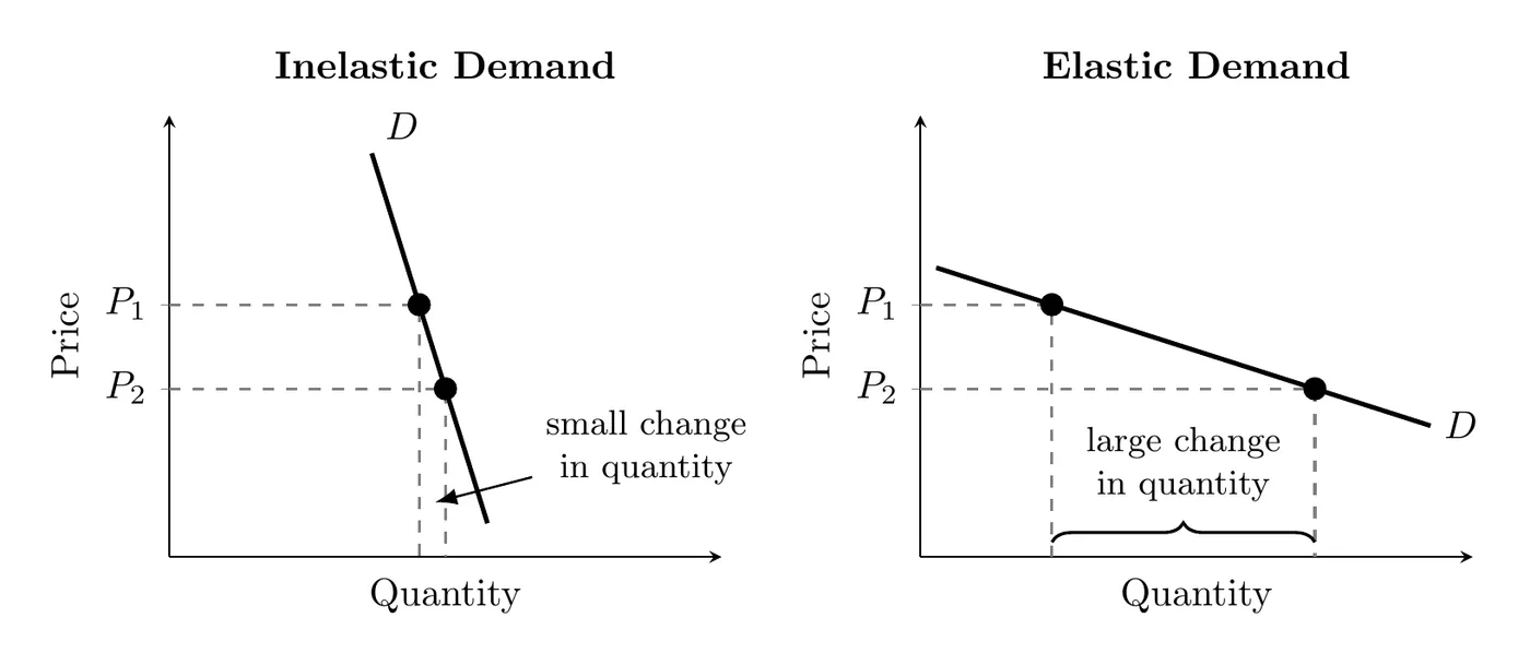
- Inelastic demand: consumers barely react, buying about the same amount even if price jumps.
- Elastic demand: consumers react a lot, a small price bump leads to a big drop in purchases.
More generally, elasticity measures how much quantity responds, in percentage terms, to a change in something else: the good’s own price (this page), consumers’ income, or the price of a related good (both on the 2.4/2.5 page). Using percentages lets you compare goods measured in totally different units, like gallons of gas and slices of pizza.
What determines elasticity
- Necessity vs. luxury: essentials like insulin have inelastic demand; non-essentials like designer shoes have elastic demand.
- Availability of substitutes: few alternatives means inelastic demand; lots of similar options (like a specific bottled water brand) means elastic demand.
- Proportion of income: cheap items that barely dent your budget (paperclips) are inelastic; expensive items (international vacations) are elastic.
- Time to adjust: demand gets more elastic over time. When gas prices jump, people still have to drive to work next week, but over a few years they can buy more fuel-efficient cars, carpool, or move closer to work.
Reading the graph
- Steep, near-vertical curves are inelastic (a big price move barely shifts quantity).
- Flat, near-horizontal curves are elastic (a small price move shifts quantity a lot).
- Perfectly inelastic is a vertical line (coefficient of 0).
- Perfectly elastic is a horizontal line (coefficient of infinity).
- Careful, slope is not elasticity. Steep vs. flat only works when you compare two curves through the same point. Along one straight-line demand curve the slope never changes, but elasticity does: demand is elastic at high prices and inelastic at low prices. The marginal revenue section and the slope example at the bottom of this page show why.
The Total Revenue Test
Total revenue (TR) equals price times quantity:
Price change | Total revenue change | Result |
Up | Down | Elastic |
Up | Up | Inelastic |
Down | Up | Elastic |
Down | Down | Inelastic |
Any change | No change | Unit elastic |
Why it works: sellers’ total revenue is the same number as buyers’ total expenditure (), so the test works for both. When demand is elastic, the percentage change in quantity is bigger than the percentage change in price, so quantity wins and revenue moves the opposite way from price. When demand is inelastic, the percentage change in price is bigger, so revenue moves the same way as price. When demand is unit elastic, the two changes are the same size and cancel out, so revenue doesn’t change.
Marginal revenue along a linear demand curve
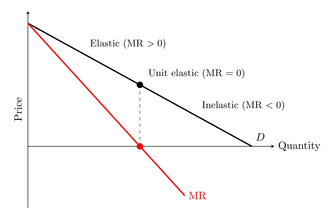
A straight-line demand curve isn’t equally elastic everywhere, it has three ranges:
- Elastic range (higher prices): marginal revenue is positive, total revenue is rising.
- Unit elastic point: marginal revenue hits zero, total revenue peaks.
- Inelastic range (lower prices): marginal revenue is negative, total revenue is falling.
Calculating the coefficient
The formula is percentage change in quantity divided by percentage change in price. Since demand is inverse, results are technically negative, but we use the absolute value:
- Greater than 1: relatively elastic
- Equal to 1: unit elastic
- The percentage changes in price and quantity are the same size (proportional), like a 10% price increase causing a 10% drop in quantity demanded.
- Less than 1: relatively inelastic
Two ways to get percentage change:
- Endpoint formula:
- Midpoint formula: (more accurate, a bit more math)
Example: price rises from $10 to $12 (a 20% increase) and quantity falls from 50 to 45 (a 10% decrease). The coefficient is , so this product is inelastic.
Check it with the Total Revenue Test: revenue goes from $10 × 50 = $500 to $12 × 45 = $540. Price went up and revenue went up, which matches inelastic demand.
Slope vs. elasticity example: take the straight-line demand curve where . Every $1 price cut adds exactly 1 unit, so the slope is the same everywhere, but elasticity isn’t:
- Price falls from $9 to $8 (an 11.1% drop) and quantity rises from 1 to 2 (a 100% increase). The coefficient is , very elastic.
- Price falls from $2 to $1 (a 50% drop) and quantity rises from 8 to 9 (a 12.5% increase). The coefficient is , inelastic.
Same slope, very different elasticity. Near the top of the curve, a $1 change is a small percentage of a high price but a big percentage of a small quantity, so demand is elastic. Near the bottom it’s the reverse.
Takeaway
Price elasticity works like an economic rubber band. When demand is elastic, pulling the price handle one way snaps total revenue the opposite way. When demand is inelastic, price and revenue move together like a rigid rope, since consumers feel they have no real choice but to pay up. Finding the unit elastic point, where marginal revenue hits zero, tells a business exactly when it’s squeezed the max revenue out of the market.