4.14 - Matrices Modeling Contexts

Overview

Lots of situations involve things switching between two states at regular time steps: customers moving between two coffee shops each week, people moving between a city and its suburbs each year, or bikes ending the day at one station or another. A transition matrix stores the switching rates. Multiply by it to step forward in time, multiply by its inverse to step backward, and multiply over and over to see where things settle in the long run.

Building a transition matrix

Here's the setup used throughout this page. A town has two coffee shops, Brew and Bean, and 1,000 regular customers. Each week:

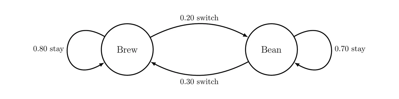
80% of Brew's customers come back to Brew, and the other 20% switch to Bean.

70% of Bean's customers come back to Bean, and the other 30% switch to Brew.

The state vector lists how many customers are in each state at one time step, written as a column. Let

\vec{x}_n

be the state vector after

n

weeks, with Brew on top and Bean on the bottom.

The transition matrix

T

has one column for each state customers come from and one row for each state they go to. The entry in row

i

, column

j

is the fraction of state

j

that moves to state

i

in one step. Write each percent as a decimal:

	From Brew	From Bean
To Brew	0.80	0.30
To Bean	0.20	0.70

T = \begin{bmatrix} 0.80 & 0.30 \\ 0.20 & 0.70 \end{bmatrix}

Each column adds up to 1, because everyone in a state has to end up somewhere (100% of Brew's customers either stay or switch). That's the quick check that the matrix is set up the right way. The rows don't need to add up to 1.

Why set it up this way? Multiply

T

by a state vector:

\begin{bmatrix} 0.80 & 0.30 \\ 0.20 & 0.70 \end{bmatrix}\begin{bmatrix} \text{Brew} \\ \text{Bean} \end{bmatrix} = \begin{bmatrix} 0.80(\text{Brew}) + 0.30(\text{Bean}) \\ 0.20(\text{Brew}) + 0.70(\text{Bean}) \end{bmatrix}

The top entry is next week's Brew customers: the 80% of Brew's customers who stayed plus the 30% of Bean's customers who switched in. The bottom entry does the same for Bean. The matrix multiplication does all the bookkeeping.

A transition diagram shows the same rates as arrows between the states:

Example 1: City and suburbs

Each year, 6% of a city's residents move to the suburbs, and 3% of suburban residents move to the city. Everyone else stays put. Write the transition matrix, with the city as the first state and the suburbs as the second.

The context gives the rates of moving. The rates of staying are what's left:

100\% - 6\% = 94\%

of city residents stay, and

100\% - 3\% = 97\%

of suburban residents stay. Columns are "from" and rows are "to":

	From City	From Suburbs
To City	0.94	0.03
To Suburbs	0.06	0.97

T = \begin{bmatrix} 0.94 & 0.03 \\ 0.06 & 0.97 \end{bmatrix}

Check:

0.94 + 0.06 = 1

and

0.03 + 0.97 = 1

Predicting future states

Multiplying the transition matrix by the current state vector gives the state one step later:

\vec{x}_{n+1} = T\vec{x}_n

To go two steps ahead, multiply by

T

twice:

\vec{x}_2 = T(T\vec{x}_0) = T^2\vec{x}_0

. In general,

\vec{x}_n = T^n\vec{x}_0

On a TI-84, store

T

as [A] and the starting state vector as [B] (a

2 \times 1

matrix), then compute [A]^n*[B] with your value of

n

. Here

T^n

means multiplying the matrix by itself

n

times, not raising each entry to the

n

th power.

Example 2: Two weeks ahead

This week (week 0), Brew and Bean each have 500 customers. Predict the number of customers at each shop next week and two weeks from now.

Next week:

\vec{x}_1 = T\vec{x}_0 = \begin{bmatrix} 0.80 & 0.30 \\ 0.20 & 0.70 \end{bmatrix}\begin{bmatrix} 500 \\ 500 \end{bmatrix} = \begin{bmatrix} 400 + 150 \\ 100 + 350 \end{bmatrix} = \begin{bmatrix} 550 \\ 450 \end{bmatrix}

Two weeks from now:

\vec{x}_2 = T\vec{x}_1 = \begin{bmatrix} 0.80 & 0.30 \\ 0.20 & 0.70 \end{bmatrix}\begin{bmatrix} 550 \\ 450 \end{bmatrix} = \begin{bmatrix} 440 + 135 \\ 110 + 315 \end{bmatrix} = \begin{bmatrix} 575 \\ 425 \end{bmatrix}

You get the same result from

T^2\vec{x}_0

in one step:

T^2 = \begin{bmatrix} 0.70 & 0.45 \\ 0.30 & 0.55 \end{bmatrix}, \qquad T^2\begin{bmatrix} 500 \\ 500 \end{bmatrix} = \begin{bmatrix} 350 + 225 \\ 150 + 275 \end{bmatrix} = \begin{bmatrix} 575 \\ 425 \end{bmatrix}

Answer: the model predicts 550 Brew customers and 450 Bean customers next week, and 575 Brew customers and 425 Bean customers in two weeks. The total stays at 1,000, as it should, since customers only move between the two shops.

The steady state

Keep multiplying by

T

week after week and watch the numbers. (The model can give fractions of a customer. Think of them as averages, and round only when you report an answer.)

Week $n$	0	1	2	3	4	5
Brew	500	550	575	587.5	593.75	596.875
Bean	500	450	425	412.5	406.25	403.125

Brew's count keeps climbing toward 600 and Bean's keeps falling toward 400, and each week the gap is cut in half.

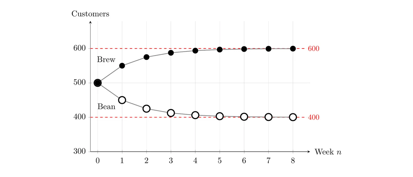
That leveling off is the steady state: a distribution between the states that doesn't change from one step to the next. In symbols, a steady state

\vec{s}

satisfies

T\vec{s} = \vec{s}

Check it here:

\begin{bmatrix} 0.80 & 0.30 \\ 0.20 & 0.70 \end{bmatrix}\begin{bmatrix} 600 \\ 400 \end{bmatrix} = \begin{bmatrix} 480 + 120 \\ 120 + 280 \end{bmatrix} = \begin{bmatrix} 600 \\ 400 \end{bmatrix}

Customers haven't stopped switching. Each week, 20% of 600, or 120 customers, leave Brew for Bean, and 30% of 400, also 120 customers, leave Bean for Brew. The two flows cancel out, so the totals stay put.

There are two ways to find a steady state:

Repeated multiplication (technology): compute $T^n\vec{x}_0$ for a large $n$ . Here $T^{20}\vec{x}_0 \approx \begin{bmatrix} 600 \\ 400 \end{bmatrix}$ , and larger values of $n$ give the same thing.

Algebra: call the steady state $\begin{bmatrix} a \\ b \end{bmatrix}$ . The top row of $T\vec{s} = \vec{s}$ says $0.80a + 0.30b = a$ , which simplifies to $0.30b = 0.20a$ , or $b = \frac{2}{3}a$ . The total is fixed at 1,000, so $a + \frac{2}{3}a = 1000$ , which gives $a = 600$ and $b = 400$ .

For transition matrices like this one, where every entry is positive, the steady state doesn't depend on where you start. Even if all 1,000 customers started at Brew, the model would still head to 600 and 400. Only the total matters, which is why a steady state is often given as percents: in the long run, about 60% of the customers go to Brew and 40% go to Bean.

Predicting past states

Since

\vec{x}_{n+1} = T\vec{x}_n

, you can go backward by undoing the multiplication with the inverse matrix from Topic 4.11:

\vec{x}_n = T^{-1}\vec{x}_{n+1}

Each multiplication by

T^{-1}

steps one time period into the past. To go back

k

steps, multiply by

T^{-1}

a total of

k

times.

Example 3: Going back in time

Brew and Bean each have 500 customers this week. How many customers did each shop have last week? Two weeks ago?

Step 1: Find

T^{-1}

. The determinant is

\det(T) = (0.80)(0.70) - (0.30)(0.20) = 0.56 - 0.06 = 0.5

, so

T^{-1} = \frac{1}{0.5}\begin{bmatrix} 0.70 & -0.30 \\ -0.20 & 0.80 \end{bmatrix} = \begin{bmatrix} 1.4 & -0.6 \\ -0.4 & 1.6 \end{bmatrix}

Step 2: Multiply this week's state by

T^{-1}

to get last week's.

T^{-1}\begin{bmatrix} 500 \\ 500 \end{bmatrix} = \begin{bmatrix} 700 - 300 \\ -200 + 800 \end{bmatrix} = \begin{bmatrix} 400 \\ 600 \end{bmatrix}

Step 3: Do it again to get two weeks ago.

T^{-1}\begin{bmatrix} 400 \\ 600 \end{bmatrix} = \begin{bmatrix} 560 - 360 \\ -160 + 960 \end{bmatrix} = \begin{bmatrix} 200 \\ 800 \end{bmatrix}

Check by going forward one week from last week's numbers:

T\begin{bmatrix} 400 \\ 600 \end{bmatrix} = \begin{bmatrix} 320 + 180 \\ 80 + 420 \end{bmatrix} = \begin{bmatrix} 500 \\ 500 \end{bmatrix}

Answer: last week, Brew had 400 customers and Bean had 600. Two weeks ago, Brew had 200 and Bean had 800.

Notice that

T^{-1}

has negative entries, so it isn't a transition matrix itself. It's only a tool for undoing one. That also means going back too far can give impossible answers. One more step back gives

T^{-1}\begin{bmatrix} 200 \\ 800 \end{bmatrix} = \begin{bmatrix} -200 \\ 1200 \end{bmatrix}

, a negative number of customers. The model can't explain this week's numbers that far back, so the backward predictions stop making sense after two weeks. Always check that a past state is realistic.

Example 4: Bike-share stations

A bike-share program has 200 bikes and two stations, North and South. Each day, 70% of the bikes that start at North end the day at North, and the rest end at South. Of the bikes that start at South, 20% end the day at North and the rest end at South. This morning, 140 bikes are at North and 60 are at South.

(a) Write the transition matrix $T$ , with North as the first state.

(b) Predict the number of bikes at each station after one day and after two days.

(d) Find the steady state and explain what it means for the program.

(a) The rates of staying are 70% at North and

100\% - 20\% = 80\%

at South:

T = \begin{bmatrix} 0.70 & 0.20 \\ 0.30 & 0.80 \end{bmatrix}

Both columns add up to 1.

(b) Multiply once, then again:

T\begin{bmatrix} 140 \\ 60 \end{bmatrix} = \begin{bmatrix} 98 + 12 \\ 42 + 48 \end{bmatrix} = \begin{bmatrix} 110 \\ 90 \end{bmatrix} \qquad T\begin{bmatrix} 110 \\ 90 \end{bmatrix} = \begin{bmatrix} 77 + 18 \\ 33 + 72 \end{bmatrix} = \begin{bmatrix} 95 \\ 105 \end{bmatrix}

After one day, the model predicts 110 bikes at North and 90 at South. After two days, it predicts 95 at North and 105 at South.

(c)

\det(T) = (0.70)(0.80) - (0.20)(0.30) = 0.5

, so

T^{-1} = \frac{1}{0.5}\begin{bmatrix} 0.80 & -0.20 \\ -0.30 & 0.70 \end{bmatrix} = \begin{bmatrix} 1.6 & -0.4 \\ -0.6 & 1.4 \end{bmatrix}

T^{-1}\begin{bmatrix} 140 \\ 60 \end{bmatrix} = \begin{bmatrix} 224 - 24 \\ -84 + 84 \end{bmatrix} = \begin{bmatrix} 200 \\ 0 \end{bmatrix}

One day earlier, all 200 bikes were at North and none were at South. Check:

T\begin{bmatrix} 200 \\ 0 \end{bmatrix} = \begin{bmatrix} 140 \\ 60 \end{bmatrix}

(d) Call the steady state

\begin{bmatrix} N \\ S \end{bmatrix}

, with

N + S = 200

. The top row of

T\vec{s} = \vec{s}

gives

0.70N + 0.20S = N

, so

0.20S = 0.30N

, or

S = 1.5N

. Then

N + 1.5N = 200

, so

N = 80

and

S = 120

\text{Check: } T\begin{bmatrix} 80 \\ 120 \end{bmatrix} = \begin{bmatrix} 56 + 24 \\ 24 + 96 \end{bmatrix} = \begin{bmatrix} 80 \\ 120 \end{bmatrix}

In the long run, the model predicts about 80 bikes at North and 120 at South each day, so the program should plan for South to need more docking space than North.

Common mistakes

Putting "from" in the rows. Columns are "from" and rows are "to." If your columns don't each add up to 1, the matrix is flipped.

Using percents as whole numbers. 80% goes into the matrix as 0.80, not 80.

Multiplying in the wrong order. The next state is $T\vec{x}$ , with the matrix on the left.

Using $T$ to go backward. Past states need $T^{-1}$ . Future states use $T$ .

Raising each entry to a power. $T^3$ means $T \cdot T \cdot T$ with matrix multiplication, not cubing each entry.

Rounding too early. Keep full decimals in each state vector and round only the final answer.

Thinking the steady state means nobody switches. People still move. The numbers moving each way just balance out.

Not checking past states. A negative number in a past state means the model doesn't reach back that far.

BackNext