1.4 - Graphical Representations for One Categorical Variable

Overview

A table gives exact numbers, but a graph shows the pattern at a glance. This topic covers the two main graphs for one categorical variable, bar charts and pie charts, how to use them to justify claims in context, and how to compare two or more data sets on the same categorical variable.

Bar charts

A bar chart, also called a bar graph, displays the frequencies (counts) or relative frequencies (proportions) for the categories of a single categorical variable.

Each bar represents one category.

The height of each bar (or its length, if the bars are horizontal) shows the frequency or relative frequency of that category.

Bars are separated by gaps, because the categories are separate groups with no number line between them.

The categories can go in any order. Common choices are largest to smallest, or a natural order like Never, Sometimes, Often.

Label both axes, and start the frequency axis at 0.

A frequency bar chart and a relative frequency bar chart of the same data have exactly the same shape. Dividing every count by the same total only changes the numbers on the vertical axis.

Example 1: Making a bar chart

Make a bar chart of the homeroom data from Topic 1.3: Car 11, Bus 8, Walk 5, Bike 4, Other 2.

Step 1: Put the five categories along the horizontal axis, with space between the bars.

Step 2: Choose a scale for the vertical axis that starts at 0 and covers the largest count, 11. Going from 0 to 12 by 2s works.

Step 3: Draw each bar up to its count, and label both axes.

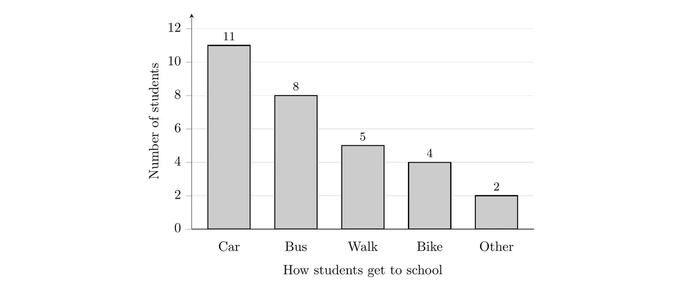
1.4 - Graphical Representations for One Categorical Variable

What it shows: Car is the most common way these 30 students get to school, followed by bus. Few students bike or get to school some other way.

Pie charts

A pie chart also displays the frequencies or relative frequencies of a categorical variable, but it shows them as parts of one whole. Each slice represents one category, and the area of each slice, as a fraction of the whole circle, equals that category's relative frequency. All the slices together make up the whole circle: a total of 1, or 100%.

To draw a slice, find its angle:

\text{angle of a slice} = \text{relative frequency} \times 360^\circ

A pie chart only works when the categories make up one whole, meaning every observational unit falls in exactly one category. If a survey says "check all that apply," the percents can add to more than 100%, and you should use a bar chart instead.

Example 2: Finding the slice angles

Find the angle of each slice in a pie chart of the homeroom data.

Each slice's angle is its relative frequency times 360°. For Car:

\frac{11}{30} \times 360^\circ = 132^\circ

A shortcut: each student is

\frac{360^\circ}{30} = 12^\circ

of the circle, so multiply each count by 12°.

How students get to school	Frequency	Relative frequency	Angle
Car	11	0.367	132°
Bus	8	0.267	96°
Walk	5	0.167	60°
Bike	4	0.133	48°
Other	2	0.067	24°
Total	30	1.001 (rounding)	360°

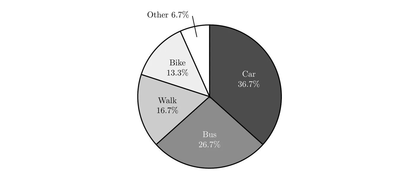
What it shows: Car and bus together make up well over half of the circle (19 of the 30 students, about 63.3%), so most of these students ride to school in a vehicle.

Bar chart or pie chart?

	Bar chart	Pie chart
Shows	Counts or relative frequencies	Relative frequencies, as parts of one whole
Best for	Comparing categories, even ones with similar sizes	Showing each category's share of the whole
Works if a unit can be in more than one category?	Yes	No
Comparing two or more data sets	Easy, with bars side by side	Harder, since slices are hard to compare

Bar charts are usually easier to read precisely, because people judge lengths better than angles or areas.

Using graphs to justify claims

A graph of a categorical variable reveals information you can use to justify claims about the variable in context. A complete justification reads specific values off the graph, compares them to what the claim says, and states a conclusion in context.

Always check the vertical axis before you trust the bar heights. If the axis doesn't start at 0, the heights aren't proportional to the frequencies, and differences look much bigger than they are.

For example, a student council asked 400 students whether they support a new schedule: 212 said yes (53%) and 188 said no (47%). Both graphs below show the same data.

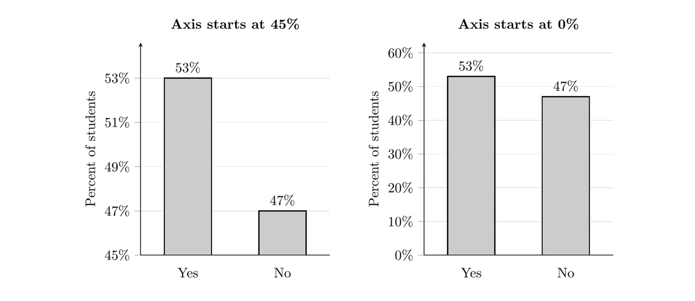
On the left, the axis starts at 45%, so the Yes bar rises 8 percentage points above the bottom of the graph and the No bar only 2. The Yes bar looks 4 times as tall, as if students overwhelmingly support the schedule. On the right, the axis starts at 0, and you can see the vote was fairly close. Base your claims on the numbers, not on how the bars look.

Comparing two or more data sets

Frequency tables, relative frequency tables, bar charts, and pie charts can all be used to compare two or more data sets on the same categorical variable.

When the data sets have different sizes, compare relative frequencies, not counts. A bigger group usually has bigger counts in every category, just because it's bigger.

A side-by-side bar chart puts the bars for each group next to each other in every category, with a key that says which group is which. Use relative frequencies on the vertical axis when the group sizes differ.

You can also draw one pie chart for each data set, but slices are harder to compare than bars.

Example 3: Two schools (AP-style)

Students at two high schools were surveyed about how they usually get to school. Northside surveyed 200 students and Southside surveyed 80.

How students get to school	Northside	Southside
Car	70	36
Bus	80	16
Walk	30	14
Bike	12	10
Other	8	4
Total	200	80

(a) A student says, "Walking is more common at Northside, since 30 Northside students walk and only 14 Southside students do." Do the data support this claim? Explain.

(b) Make a graph that compares the two distributions.

Solution

(a) No. Northside has more walkers only because it surveyed more students. Compare the proportions instead:

\text{Northside: } \frac{30}{200} = 0.15 \qquad \text{Southside: } \frac{14}{80} = 0.175

A slightly higher proportion of surveyed Southside students walk to school (17.5%) than surveyed Northside students (15%), so the data don't support the claim.

(b) Because the group sizes differ, use relative frequencies:

How students get to school	Northside	Southside
Car	0.35	0.45
Bus	0.40	0.20
Walk	0.15	0.175
Bike	0.06	0.125
Other	0.04	0.05
Total	1.00	1.00

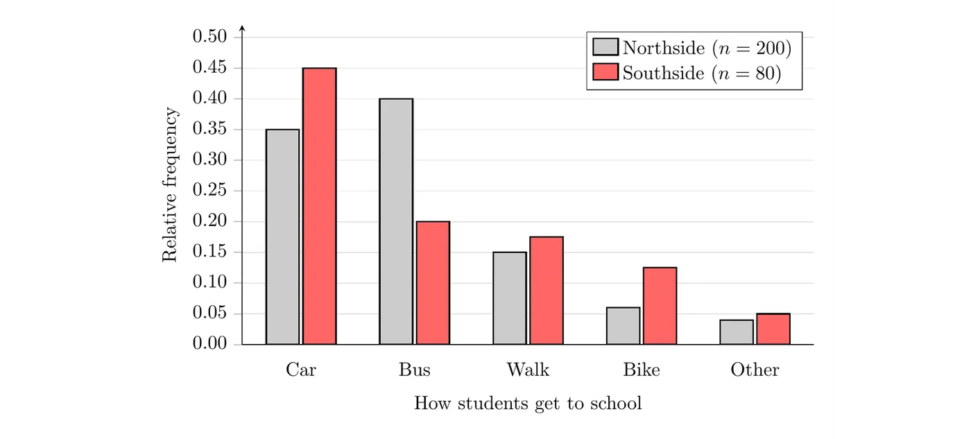
(c) Taking the bus is much more common at Northside: 0.40 of the surveyed Northside students ride the bus, twice the proportion at Southside (0.20). Southside students are more likely to come by car (0.45 compared to 0.35).

Common mistakes

Leaving out the gaps. Bars in a bar chart have gaps between them. Histograms (Topic 1.5) don't.

Starting the vertical axis above 0, or not noticing when someone else's graph does.

Using a pie chart when the categories overlap or don't make up one whole.

Comparing counts for groups of different sizes. Compare relative frequencies.

Using shape words for categorical data. Categories can go in any order, so words like "skewed" or "symmetric" don't apply to a bar chart. Describe which categories are most and least common instead.

Justifying a claim by how the graph looks. Quote the actual values from the graph.

Back Next