

1.6 - Descriptions for One Quantitative Variable Distributions
Overview
Once you've graphed a quantitative variable, the next job is to say what the graph shows. AP Statistics expects the same four things every time: shape, center, variability, and any unusual features, all in the context of the data. This topic gives you the words for each one and shows how to use a graph to support or reject a claim.
The four parts of a description
A complete description of the distribution of one quantitative variable covers:
- Shape: Is it skewed or symmetric? How many peaks does it have?
- Center: Roughly where is the middle of the data?
- Variability (spread): How spread out are the values? Where do they start and stop?
- Unusual features: Are there outliers, gaps, or clusters?
Some teachers use an acronym like SOCS (Shape, Outliers, Center, Spread) as a checklist. The acronym only reminds you what to cover. You still have to describe each part with values from the graph.
Context means naming the variable and its units. "The distribution is skewed right" is incomplete. "The distribution of commute times (in minutes) is skewed right" is what AP graders want. A response that only talks about the center is also incomplete: the exam expects all four parts, and students most often forget the unusual features. If there aren't any, say so ("there are no apparent outliers or gaps").
Shape: skewed or symmetric
Skewness describes which side of the distribution stretches out farther.
- Skewed right (positively skewed): the right tail, toward the larger values, is longer than the left. Most values are small or medium, and a few large values stretch out to the right. Incomes, home prices, and the number of texts people send in a day are usually skewed right.
- Skewed left (negatively skewed): the left tail, toward the smaller values, is longer than the right. Scores on an easy test are often skewed left: most students do well, and a few low scores stretch out to the left.
- Approximately symmetric: the left half is roughly a mirror image of the right half.
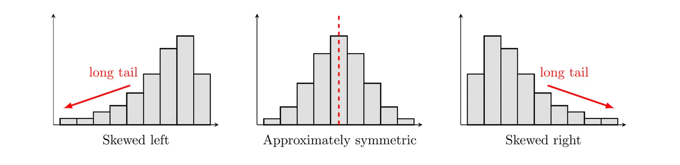
The rule to remember: the skew is named for the tail, not the peak. A skewed right distribution has its peak on the left and its long tail on the right. Also, real data is never perfectly symmetric, so write "approximately symmetric" or "roughly symmetric."
Shape: number of peaks
A peak (or mode) is a value or bar that clearly stands above its neighbors.
- Unimodal: one main peak.
- Bimodal: two prominent peaks. This often means two different groups are mixed together, like the heights of a group of 8-year-olds and their parents.
- Approximately uniform: every value or bar has about the same frequency (or relative frequency), with no prominent peaks.
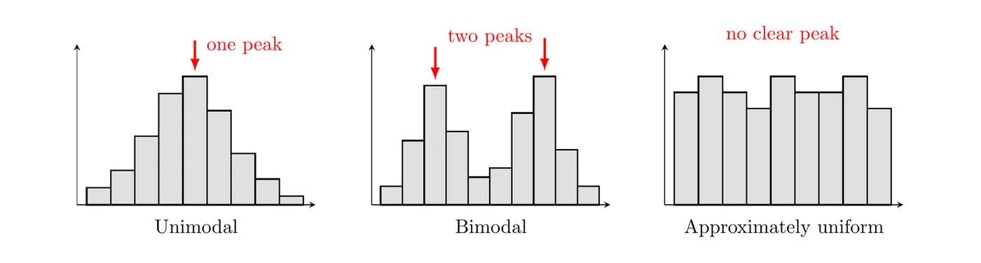
Small bumps don't count as peaks. A good shape statement usually combines both ideas, like "unimodal and skewed right" or "bimodal and roughly symmetric."
Unusual features: outliers, gaps, and clusters
- Outlier: a data value that is unusually small or large relative to the rest of the data. In this topic you spot outliers by eye. Topic 1.7 gives two rules for deciding whether a value really counts as one.
- Gap: a region between two values where there are no observed data.
- Clusters: concentrations of values, usually separated by gaps.
The dotplot below shows the ages of the 21 people at a child's birthday party. The 11 children (ages 5 to 8) form one cluster, the 9 adults (ages 31 to 41) form another, there's a gap from 8 to 31, and the one grandparent (age 68) is far from everyone else, an outlier.
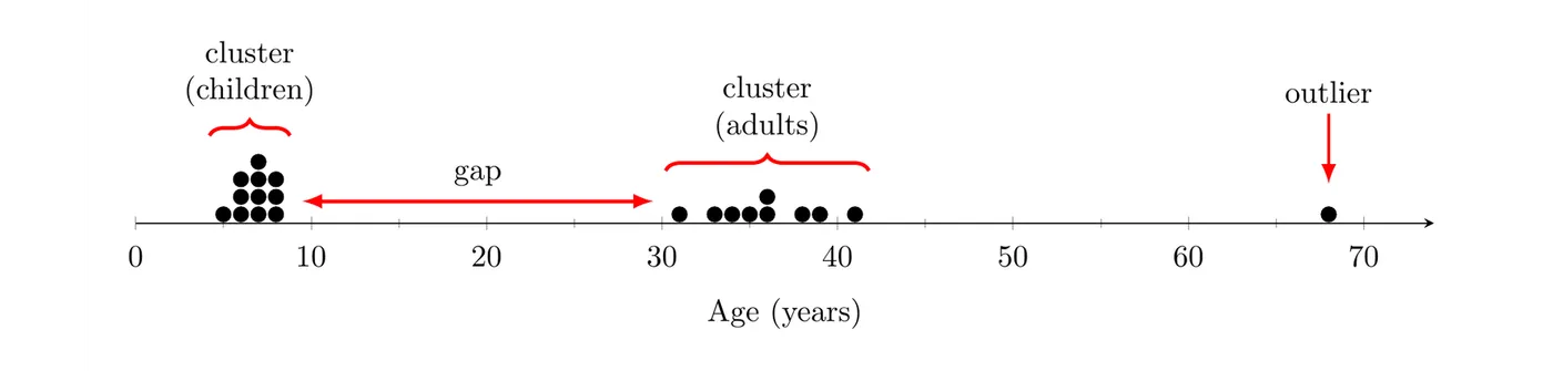
These features matter because they usually have a story. Clusters often mean the data came from different groups. An outlier might be a typing error or a genuinely special case, so investigate it instead of ignoring it.
Center and variability from a graph
Without exact data, you can still estimate the center and variability from a graph:
- Center: find the value that splits the data roughly in half. With values in order, the middle one is in position , so count dots (or bar heights) from the left until you reach it.
- Variability: say where the values run from and to, and where most of them fall.
Topic 1.7 turns these estimates into exact statistics: the mean and median for center, and the range, interquartile range, and standard deviation for variability.
Using a graph to justify a claim
A graph can reveal information that supports or contradicts a claim about the variable. To judge a claim:
- Pin down exactly what the claim says: which values, and what fraction of the data.
- Read the counts or values you need from the graph.
- Decide whether the graph supports the claim, and give the numbers as evidence, in context.
Be careful with what a graph can't show. A histogram tells you how many values fall in each bin, not the exact values, so a claim like "more than 20 students scored above 85" can't be checked from bins of width 10.
Example 1: Describing a dotplot
A librarian recorded how many books each of 25 students in a summer reading program read over the summer. Describe the distribution.
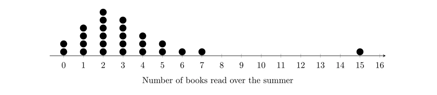
Shape: There is one peak, at 2 books. Most students read 0 to 5 books, and a few values stretch out to the right, so the distribution is unimodal and skewed right.
Center: With 25 values, the middle one is in position . Counting dots from the left: 2 students read 0 books, 4 read 1 (6 so far), and 6 read 2 (12 so far), so the 13th value is 3 books.
Variability: The values go from 0 to 15 books, and 22 of the 25 students read between 0 and 5 books.
Unusual features: Nobody read between 7 and 15 books, so there is a gap there, and the student who read 15 books looks like a high outlier.
Answer: The distribution of the number of books read over the summer by these 25 students is unimodal and skewed right, with a center of about 3 books. The number of books varies from 0 to 15, with most students reading 0 to 5. There is a gap between 7 and 15 books, and 15 books is a possible high outlier.
Example 2: Judging claims from a histogram (AP-style)
The histogram shows the scores of 80 students on a quiz. Each bin includes its left endpoint (the 80 bar is scores from 80 up to, but not including, 90), and the last bin includes 100.
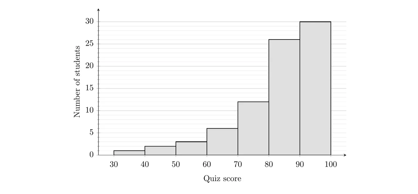
(a) Describe the shape of the distribution. (b) A teacher claims that at least 75% of the students scored 80 or higher. Does the histogram support this claim? (c) Another teacher claims that fewer than 10% of the students scored below 60. Does the histogram support this claim?
(a) The tallest bar is 90 to 100, and the bars get shorter as you move left, with a long tail stretching down to the 30s. The distribution of quiz scores is unimodal and skewed left.
(b) Add the bars at 80 and above, then divide by the total:
Only 70% of the students scored 80 or higher, which is less than 75%. The histogram does not support the claim.
(c) Add the bars below 60:
Only 7.5% of the students scored below 60, which is less than 10%. The histogram supports this claim.
Example 3: When one center doesn't tell the story
A park ranger recorded the time between 25 eruptions of a geyser, in minutes. A sign at the park says visitors usually wait about 70 minutes between eruptions. Does the stemplot support the sign?
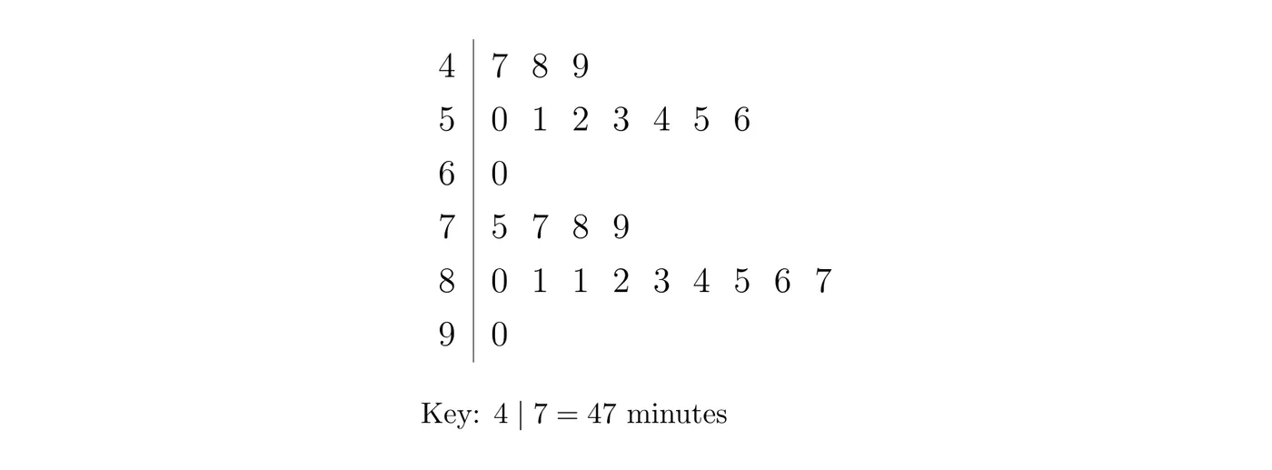
Step 1: Describe the distribution. It is bimodal, with two clusters: 11 waits from 47 to 60 minutes and 14 waits from 75 to 90 minutes. There is a gap between them: no wait was between 61 and 74 minutes.
Step 2: Check the claim. The average of all 25 waits is about 69 minutes, which is probably where "about 70" came from. But that average falls right in the gap, where none of the 25 waits landed.
Answer: The stemplot does not support the sign. Waits between eruptions tend to be either short (about 47 to 60 minutes) or long (about 75 to 90 minutes), and a wait of about 70 minutes never happened in this sample. For a bimodal distribution, describe each cluster instead of giving one center.
Common mistakes
- Naming the skew after the peak. A peak on the left with a long tail on the right is skewed right.
- Leaving out context. Name the variable and its units in every description.
- Skipping unusual features. If there are no outliers, gaps, or clusters, say that.
- Calling a distribution "normal" because it looks mound-shaped. Say "approximately symmetric and unimodal." The normal distribution is a specific model you'll meet in Unit 2.
- Describing the bars instead of the data, like "the bars go up and then down."
- Giving one center for a bimodal distribution as if it described a typical value.