1.7 - Summary Statistics for One Quantitative Variable

Overview

Topic 1.6 described distributions in words. This topic puts numbers on them: measures of center (mean and median), measures of position (quartiles and percentiles), and measures of variability (range, interquartile range, and standard deviation). You'll also see how changing units changes these numbers, two rules for identifying outliers, and how to choose and compare summary statistics.

Most of this page uses one small data set. Suppose Ms. Lee asked 9 students how many minutes they spent on homework last night:

22, \; 48, \; 15, \; 25, \; 31, \; 12, \; 20, \; 25, \; 18

In order from smallest to largest:

12, \; 15, \; 18, \; 20, \; 22, \; 25, \; 25, \; 31, \; 48

Measures of center: mean and median

The two most common measures of center are the mean and the median.

The mean

The mean is the sum of all the values divided by the number of values. For a sample, the mean is written

\bar{x}

("x-bar"):

\bar{x} = \frac{1}{n}\sum_{i=1}^{n} x_i = \frac{x_1 + x_2 + \cdots + x_n}{n}

Here

x_i

is the

i

th data value and

n

is the number of values. (The mean of a whole population is written

\mu

, the Greek letter mu.) For the homework data:

\bar{x} = \frac{12 + 15 + 18 + 20 + 22 + 25 + 25 + 31 + 48}{9} = \frac{216}{9} = 24

In context: the mean time these 9 students spent on homework was 24 minutes. The mean is the balance point of the distribution: put a weight at each value on a number line, and it balances at the mean.

The median

The median is the middle value when the data are in order. With

n

values, the median is in position

\frac{n+1}{2}

Odd number of values: the median is the single middle value. For the 9 homework times, it's the 5th value, 22 minutes.

Even number of values: the median is the mean of the two middle values. If a 10th student reported 30 minutes, the ordered data would be 12, 15, 18, 20, 22, 25, 25, 30, 31, 48, and the median would be $\frac{22 + 25}{2} = 23.5$ minutes.

In context: about half of the 9 students spent 22 minutes or less on homework, and about half spent 22 minutes or more.

In an ordered data set, the smallest value is the minimum and the largest is the maximum. For the homework data, the minimum is 12 minutes and the maximum is 48 minutes.

Measures of position: quartiles and percentiles

The first quartile,

Q_1

, is the median of the lower half of the ordered data, and the third quartile,

Q_3

, is the median of the upper half. About 25% of the values are at or below

Q_1

, and about 75% are at or below

Q_3

. The median is the second quartile,

Q_2

. Together,

Q_1

and

Q_3

mark off the middle 50% of the data.

When

n

is odd, leave the median itself out of both halves. This is the method the TI-84 uses. (Some software splits the data a little differently and gets slightly different quartiles.)

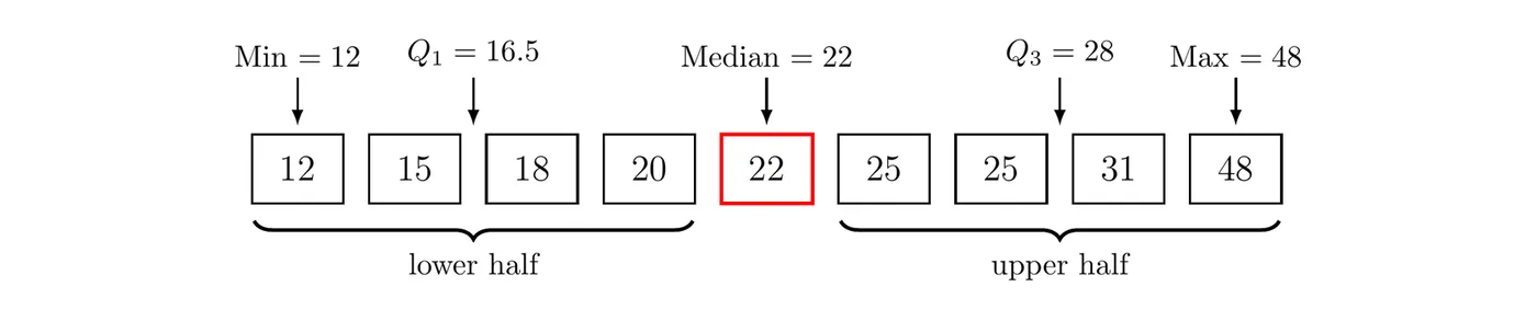
1.7 - Summary Statistics for One Quantitative Variable

Q_1 = \frac{15 + 18}{2} = 16.5 \qquad Q_3 = \frac{25 + 31}{2} = 28

In context: about 25% of these students spent 16.5 minutes or less on homework, and about 75% spent 28 minutes or less.

More generally, the

p

th percentile is the value with

p

% of the data at or below it.

Q_1

is the 25th percentile, the median is the 50th, and

Q_3

is the 75th. To find the percentile of a value, find the percent of the data at or below it. For example, 7 of the 9 homework times are 25 minutes or less, and

\frac{7}{9} \approx 0.78

, so a student who spent 25 minutes is at about the 78th percentile.

Measures of variability

Three common measures of variability (spread) are the range, the interquartile range, and the standard deviation. Larger values mean the data are more spread out.

Range

The range is the maximum minus the minimum. For the homework data, the range is

48 - 12 = 36

minutes. It's easy to find, but it depends only on the two most extreme values.

Interquartile range (IQR)

The interquartile range is

\text{IQR} = Q_3 - Q_1

, the spread of the middle 50% of the data. For the homework data,

\text{IQR} = 28 - 16.5 = 11.5

minutes. In context: the middle half of the homework times spans 11.5 minutes.

Standard deviation

The standard deviation measures a typical distance of the data values from their mean. For a sample, it is written

s

s = \sqrt{\frac{1}{n-1}\sum_{i=1}^{n}(x_i - \bar{x})^2}

The square of the standard deviation,

s^2

, is called the sample variance. To find

s

by hand:

Find the mean $\bar{x}$ .

Find each deviation $x_i - \bar{x}$ (how far each value is from the mean).

Square each deviation and add them up.

Divide by $n - 1$ . This is the variance $s^2$ .

Take the square root to get $s$ .

Why square? The deviations always add up to 0 (values above the mean balance the ones below), so squaring makes every deviation count as a positive amount. Dividing by

n - 1

instead of

n

makes

s^2

a better estimate of the population's variance.

Example 1: Standard deviation by hand

Five friends own 1, 3, 4, 4, and 8 pets. Find and interpret the standard deviation.

Step 1: The mean is

\bar{x} = \frac{1 + 3 + 4 + 4 + 8}{5} = \frac{20}{5} = 4

pets.

Step 2: Find each deviation and its square.

$x_i$	$x_i - \bar{x}$	$(x_i - \bar{x})^2$
1	$-3$	9
3	$-1$	1
4	0	0
4	0	0
8	4	16
Sum	0	26

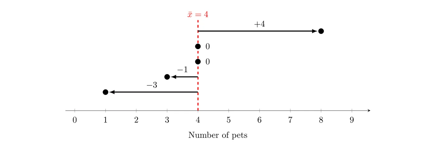
Step 3: Divide by

n - 1 = 4

, then take the square root.

s^2 = \frac{26}{4} = 6.5 \qquad s = \sqrt{6.5} \approx 2.55

Answer: The number of pets these 5 friends own typically varies by about 2.55 pets from the mean of 4 pets.

The standard deviation is never negative, equals 0 only when every value is the same, and has the same units as the data.

TI-84: press STAT, choose 1:Edit, and enter the data in L1. Then press STAT, go to CALC, and choose 1:1-Var Stats with List set to L1. You get

\bar{x}

, Sx (the sample standard deviation

s

, the one you want), σx (the population version),

n

, and minX, Q1, Med, Q3, and maxX. For the homework data, Sx

\approx 10.65

minutes.

Changing units of measurement

Changing the units of a variable changes its summary statistics in a predictable way. Suppose every value is converted with

\text{new} = a + b \cdot \text{old}

, where

a

and

b

are constants (and

b > 0

Statistic	Adding $a$ to every value	Multiplying every value by $b$
Mean, median, quartiles, percentiles, min, max	Add $a$	Multiply by $b$
Range, IQR, standard deviation	No change	Multiply by $b$
Variance	No change	Multiply by $b^2$
Shape	No change	No change

Adding a constant slides every value the same distance, so the center moves but the distances between values (the spread) don't change. Multiplying stretches or shrinks the whole number line, so both change. Neither changes the shape.

Example 2: Converting temperatures

Suppose the daily high temperatures in a city for one month have a mean of 20.0°C, a median of 19.0°C, a minimum of 11.0°C, a standard deviation of 4.0°C, and an IQR of 5.5°C. Find each statistic in degrees Fahrenheit, using

F = 1.8C + 32

Center and position (multiply by 1.8, then add 32):

\text{mean} = 1.8(20.0) + 32 = 68.0 \qquad \text{median} = 1.8(19.0) + 32 = 66.2 \qquad \text{min} = 1.8(11.0) + 32 = 51.8

Spread (multiply by 1.8 only):

s = 1.8(4.0) = 7.2 \qquad \text{IQR} = 1.8(5.5) = 9.9

Answer: In Fahrenheit, the mean is 68.0°F, the median is 66.2°F, the minimum is 51.8°F, the standard deviation is 7.2°F, and the IQR is 9.9°F. Adding 32 shifts every temperature without spreading them out, so it doesn't affect

s

or the IQR. (The variance becomes

7.2^2 = 51.84

squared degrees.)

Identifying outliers

There are many methods for identifying possible outliers. Two are used most often, and you should know both.

The 1.5 × IQR rule

A value is an outlier if it is more than

1.5 \times \text{IQR}

above

Q_3

or more than

1.5 \times \text{IQR}

below

Q_1

. The two cutoffs are often called fences:

\text{lower fence} = Q_1 - 1.5 \times \text{IQR} \qquad \text{upper fence} = Q_3 + 1.5 \times \text{IQR}

For the homework data,

1.5 \times 11.5 = 17.25

, so the fences are

16.5 - 17.25 = -0.75

and

28 + 17.25 = 45.25

. The value 48 is above 45.25, so 48 minutes is an outlier. No value is below

-0.75

The 2 standard deviations rule

A value is an outlier if it is more than 2 standard deviations above or below the mean, that is, above

\bar{x} + 2s

or below

\bar{x} - 2s

. For the homework data,

24 \pm 2(10.65)

gives about 2.7 to 45.3 minutes. Again, 48 is outside, so it's an outlier by this rule too.

Example 3: When the two rules disagree

The ages of the 10 people in a Saturday yoga class are 29, 32, 35, 36, 37, 38, 41, 42, 59, and 60. Check for outliers with both rules.

1.5 × IQR rule: The lower half is 29, 32, 35, 36, 37, so

Q_1 = 35

. The upper half is 38, 41, 42, 59, 60, so

Q_3 = 42

\text{IQR} = 42 - 35 = 7 \qquad 1.5 \times 7 = 10.5

\text{fences: } 35 - 10.5 = 24.5 \quad \text{and} \quad 42 + 10.5 = 52.5

Both 59 and 60 are above 52.5, so both are outliers by this rule.

2 standard deviations rule: The calculator gives

\bar{x} = 40.9

and

s \approx 10.525

years, so

2s \approx 21.05

40.9 - 21.05 = 19.85 \qquad 40.9 + 21.05 = 61.95

Every age is between 19.85 and 61.95, so this rule finds no outliers.

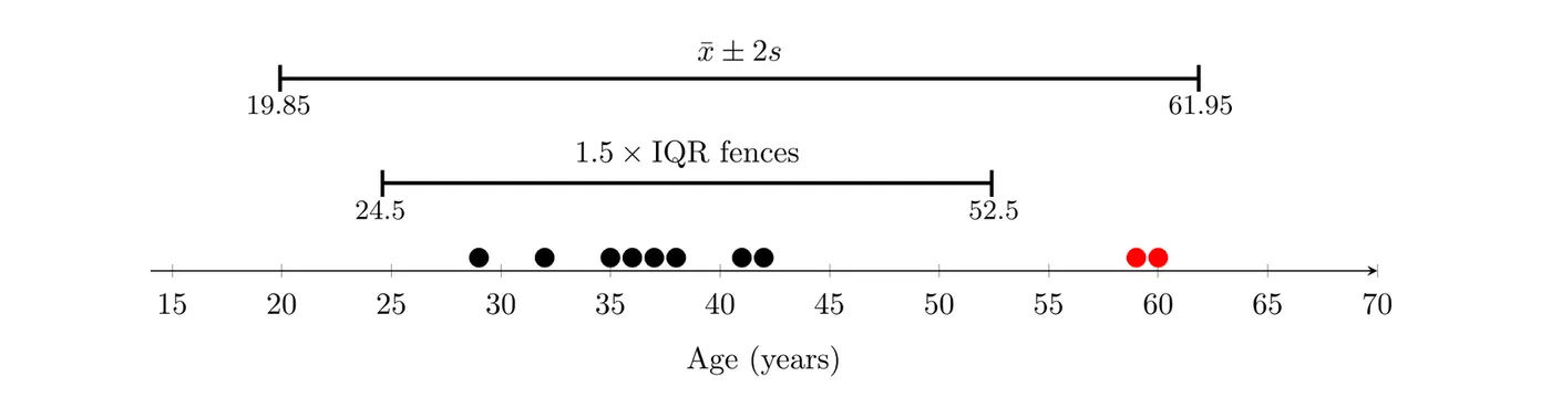
Why they disagree: the two oldest people pull the mean up and make

s

much larger, which stretches the

\bar{x} \pm 2s

interval wide enough to include them. The quartiles barely move, so the 1.5 × IQR rule still catches them. If a question names a rule, use it. If not, name the rule you chose and show the numbers. The 1.5 × IQR rule is the more common choice, and it's the one boxplots use (Topic 1.8).

Resistant and nonresistant statistics

A statistic is resistant (or robust) if outliers don't affect it much, if at all. The median and IQR are resistant. The mean, standard deviation, and range are nonresistant: one extreme value can change them a lot.

To see this, suppose the 48 in the homework data had been typed as 480 by mistake:

Statistic	Original data (48)	With the typo (480)
Mean	24 minutes	72 minutes
Standard deviation	10.65 minutes	153.11 minutes
Range	36 minutes	468 minutes
Median	22 minutes	22 minutes
IQR	11.5 minutes	11.5 minutes

The mean tripled and the standard deviation exploded, while the median and IQR didn't change at all. The median depends only on which value is in the middle, and the quartiles only on the values near the 25% and 75% marks.

Choosing a summary statistic

Roughly symmetric with no outliers: report the mean and standard deviation. They use every value.

Strongly skewed, or with outliers: report the median and IQR. They aren't pulled around by the extreme values, so they describe a typical value and a typical spread better.

On the AP exam, justify the choice with the shape: "Because the distribution is skewed right with a high outlier, the median and IQR are better summaries. They are resistant, while the mean and standard deviation are pulled toward the outlier." This is why news reports give the median home price: home prices are skewed right, and a few mansions would pull the mean far above what a typical home costs.

Comparing summary statistics

Summary statistics let you compare two or more independent samples on center, variability, shape, and outliers, and they can be evidence for or against a claim about the variable.

Example 4: Comparing wait times (AP-style)

A coffee shop owner timed the wait for random samples of 40 customers at each of two locations. The summary statistics, in minutes, are below.

Location	$n$	Mean	SD	Min	$Q_1$	Median	$Q_3$	Max
A	40	4.2	1.1	1.8	3.5	4.1	4.9	6.8
B	40	5.6	3.4	0.9	3.0	4.4	7.2	16.5

(a) Compare the distributions of wait times at the two locations. (b) The owner claims that customers at Location B usually wait longer than customers at Location A. Do the statistics support this claim?

(a) Center: The medians are close: 4.4 minutes at B and 4.1 minutes at A. The means are farther apart (5.6 versus 4.2 minutes) because a few very long waits pull B's mean up.

Variability: B's wait times are much more variable. B's IQR is

7.2 - 3.0 = 4.2

minutes, three times A's IQR of

4.9 - 3.5 = 1.4

minutes, and B's standard deviation (3.4 minutes) is about three times A's (1.1 minutes).

Shape: At A, the mean (4.2) is about equal to the median (4.1), and

Q_1

and

Q_3

are about equally far from the median, so A's distribution is roughly symmetric. At B, the mean is well above the median, and

Q_3

is 2.8 minutes above the median while

Q_1

is only 1.4 minutes below it, so B's distribution is skewed right. (Topic 1.8 explains this link between the mean, median, and shape.)

Outliers (1.5 × IQR rule):

\text{A: } 3.5 - 1.5(1.4) = 1.4 \quad \text{and} \quad 4.9 + 1.5(1.4) = 7.0

\text{B: } 3.0 - 1.5(4.2) = -3.3 \quad \text{and} \quad 7.2 + 1.5(4.2) = 13.5

A's min (1.8) and max (6.8) are inside its fences, so A has no outliers. B's max of 16.5 minutes is above 13.5, so B has at least one high outlier.

(b) The statistics only partly support the claim. A typical customer waits about the same at both locations (medians of 4.1 and 4.4 minutes). What's different is long waits: about a quarter of B's customers waited 7.2 minutes or more (

Q_3 = 7.2

), while no customer at A waited longer than 6.8 minutes. A fair summary: B's typical wait is only slightly longer, but long waits are much more common at B.

Common mistakes

Using σx instead of Sx from 1-Var Stats when the data are a sample.

Finding the median or quartiles without putting the data in order first.

Including the median in both halves when finding $Q_1$ and $Q_3$ for an odd number of values.

Adding the constant to the standard deviation or IQR when converting units. Adding shifts the center only.

Reporting the IQR as an interval ("16.5 to 28"). The IQR is one number: $28 - 16.5 = 11.5$ .

Calling a value an outlier because it "looks far away." Show the fences or the $\bar{x} \pm 2s$ cutoffs.

Summarizing skewed data, or data with outliers, with the mean and standard deviation.

Back Next