1.9 - Comparisons of the Distributions for One Quantitative Variable

Overview

Many statistical questions compare groups. Do athletes have lower resting pulse rates? Does one battery last longer than another? This topic shows how to compare distributions with graphs and summary statistics, how to use a comparison to support a claim, and how

z

-scores let you compare individual values, even values from different distributions.

How to write a comparison

Compare the same four features as in Topic 1.6: shape, center, variability, and unusual features (outliers, clusters, gaps). Three rules make a comparison earn full credit:

Use comparison words like "greater than," "less than," or "about the same as." Two separate descriptions placed side by side don't count as a comparison.

Back it up with numbers: medians, IQRs, ranges, means, standard deviations, or values read from the graph.

Keep the context: name the variable, the units, and the groups.

For example: "The median flight distance for the Dart (8 meters) is greater than the median for the Glider (5 meters)."

Graphs for comparing distributions

Histograms, back-to-back stemplots, and dotplots can compare center, variability, shape, outliers, clusters, and gaps. Boxplots can compare center, variability, outliers, and skewness (or symmetry), but not clusters, gaps, or peaks.

Graph	How to set it up	Best for
Parallel dotplots	One dotplot per group, stacked on the same scale	Small data sets; shows every value, clusters, and gaps
Back-to-back stemplot	Shared stems in the middle, one group's leaves on each side	Two small data sets; shows shape and individual values
Histograms	Stacked, with the same scale on both axes	Larger data sets; shows shape
Parallel boxplots	One boxplot per group on the same number line	Any size; quick comparison of center, spread, outliers, and skew

Whatever you use, put the groups on the same scale. If the groups have different sizes, compare histograms with relative frequencies (proportions) rather than counts. And a comparison of graphs can always include numerical summaries, like the mean and standard deviation, as extra evidence.

Example 1: Comparing dotplots

A class tested two paper airplane designs, the Dart and the Glider, by flying each one 20 times and measuring the distance in meters. Compare the distributions.

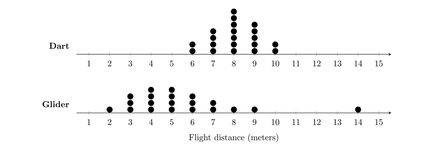
1.9 - Comparisons of the Distributions for One Quantitative Variable

Shape: The Dart's distances are roughly symmetric with a peak at 8 meters. The Glider's are skewed right, with most flights between 3 and 6 meters.

Center: With 20 flights each, the median is the mean of the 10th and 11th values. Counting dots, the Dart's median is 8 meters and the Glider's is 5 meters.

Variability: The Dart's range is

10 - 6 = 4

meters and the Glider's is

14 - 2 = 12

meters. Even without the 14-meter flight, the Glider's distances span 2 to 9 meters.

Unusual features: The Glider has a gap between 9 and 14 meters, and 14 meters is an outlier (its quartiles are 4 and 6.5, so the upper fence is

6.5 + 1.5(2.5) = 10.25

). The Dart has no outliers or gaps.

Answer: The Dart's flight distances are roughly symmetric, while the Glider's are skewed right. The Dart tends to fly farther (median 8 m versus 5 m), and its distances are much more consistent (range 4 m versus 12 m). The Glider has a high outlier at 14 m, separated from its other flights by a gap, and the Dart has no unusual features.

Example 2: Comparing a back-to-back stemplot

A health class measured the resting pulse rates, in beats per minute (bpm), of 15 athletes and 15 non-athletes. (a) Compare the distributions. (b) Does the stemplot support the claim that athletes tend to have lower resting pulse rates?

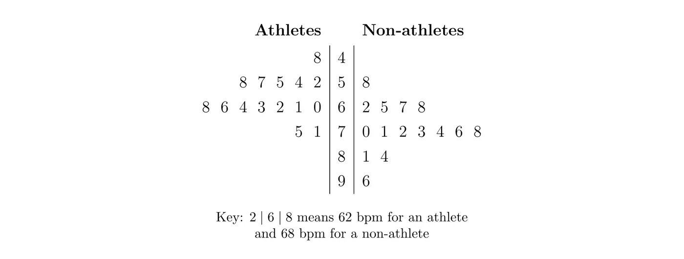
Reading the leaves (on the athletes' side, they increase as you move away from the stem), the five-number summaries are:

Group	Min	$Q_1$	Median	$Q_3$	Max
Athletes	48	55	61	66	75
Non-athletes	58	67	72	78	96

(a) Shape: Both distributions are roughly symmetric and unimodal, apart from one high value among the non-athletes.

Center: The athletes' median pulse (61 bpm) is lower than the non-athletes' (72 bpm).

Variability: The IQRs are equal (11 bpm each), so the middle halves are equally spread out. The non-athletes' range (38 bpm) is larger than the athletes' (27 bpm), mostly because of that one high value.

Unusual features: For the non-athletes, the upper fence is

78 + 1.5(11) = 94.5

, so 96 bpm is an outlier. The athletes' fences are

55 - 16.5 = 38.5

and

66 + 16.5 = 82.5

, so they have no outliers.

(b) Yes. The athletes' median is 11 bpm lower, and 14 of the 15 athletes have pulse rates below 72 bpm, the non-athletes' median. These are just two groups that were observed, though, so the stemplot can't show that exercise causes lower pulse rates. That takes an experiment (Topic 1.13).

Example 3: Parallel boxplots and a claim (AP-style)

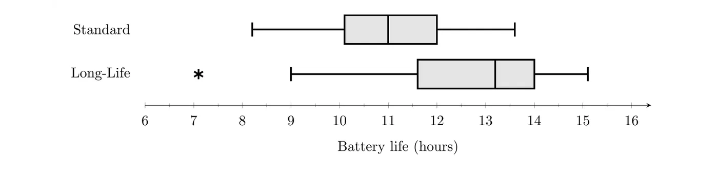
A company tested random samples of 50 Standard batteries and 50 Long-Life batteries, recording how many hours each lasted in continuous use.

Type	Mean	SD	Min	$Q_1$	Median	$Q_3$	Max
Standard	11.0	1.3	8.2	10.1	11.0	12.0	13.6
Long-Life	12.7	1.6	7.1	11.6	13.2	14.0	15.1

(a) Compare the distributions of battery life. (b) The company wants to advertise that Long-Life batteries last longer. Use the boxplots to support or refute this claim.

(a) Shape: Standard battery life is roughly symmetric: the median is near the middle of the box, the whiskers are similar in length, and the mean equals the median (11.0 hours). Long-Life battery life is skewed left: the median (13.2) is closer to

Q_3

, the left whisker is longer, there's a low outlier, and the mean (12.7) is less than the median.

Center: The median life of Long-Life batteries (13.2 hours) is 2.2 hours greater than that of Standard batteries (11.0 hours).

Variability: Long-Life batteries are a bit more variable: their IQR is

14.0 - 11.6 = 2.4

hours versus

12.0 - 10.1 = 1.9

hours, and their standard deviation is 1.6 hours versus 1.3 hours.

Unusual features: One Long-Life battery lasted only 7.1 hours, below its lower fence of

11.6 - 1.5(2.4) = 8.0

, so it's an outlier. The Standard batteries have no outliers (fences 7.25 and 14.85).

(b) The boxplots support the claim. The Long-Life

Q_1

(11.6 hours) is greater than the Standard median (11.0 hours), so about 75% of the Long-Life batteries lasted more than 11.6 hours, while only about half of the Standard batteries lasted more than 11.0 hours. The Long-Life median (13.2) is even above the Standard

Q_3

(12.0). One caution for the ad: the shortest-lived battery in either sample was a Long-Life battery (7.1 hours). Whether a difference this size could be due to chance in random sampling is a question for inference (Unit 4).

Standardized scores (z-scores)

Sometimes you want to know how unusual one value is, not compare whole distributions. A standardized score, or

z

-score, measures how many standard deviations a data value is above or below the mean:

z = \frac{x_i - \mu}{\sigma}

Here

x_i

is the data value,

\mu

is the population mean, and

\sigma

is the population standard deviation. When the population mean and standard deviation are unknown, use the sample statistics instead:

z = \frac{x_i - \bar{x}}{s}

A positive $z$ -score means the value is above the mean, and a negative one means it's below. A $z$ -score of 0 means the value equals the mean.

A $z$ -score has no units: the units cancel in the fraction. That's what lets you compare values measured on different scales.

The 2 standard deviations rule from Topic 1.7 says a value is an outlier when $z > 2$ or $z < -2$ . For the yoga class, the 60-year-old has $z = \frac{60 - 40.9}{10.525} \approx 1.81$ , which is why that rule didn't flag this age.

To interpret a

z

-score, use this template: "The value is ___ standard deviations above (or below) the mean ___ (in context)."

Example 4: Calculating z-scores

Suppose the heights of adult women in a population have mean

\mu = 64

inches and standard deviation

\sigma = 2.7

inches. (a) Find and interpret the

z

-score of a woman who is 70 inches tall. (b) Do the same for a woman who is 60 inches tall. (c) What height has a

z

-score of

-0.5

(a)

z = \frac{70 - 64}{2.7} = \frac{6}{2.7} \approx 2.22

A height of 70 inches is about 2.22 standard deviations above the mean height of 64 inches.

(b)

z = \frac{60 - 64}{2.7} = \frac{-4}{2.7} \approx -1.48

A height of 60 inches is about 1.48 standard deviations below the mean. Within this one distribution, 70 inches is the more unusual height, since it's farther from the mean in standard deviations.

(c) Solve the formula for

x

x = \mu + z\sigma

x = 64 + (-0.5)(2.7) = 64 - 1.35 = 62.65

A woman 62.65 inches tall is half a standard deviation below the mean.

Comparing z-scores

z

-scores compare the relative positions of values within one distribution or between different distributions. A raw score only means something next to its own mean and spread, and the

z

-score builds both in.

Example 5: Who did better? (AP-style)

Maya scored 84 on her biology exam, where the class mean was 76 and the standard deviation was 4. Jordan scored 88 on his history exam, where the class mean was 80 and the standard deviation was 5. Relative to their classes, who did better?

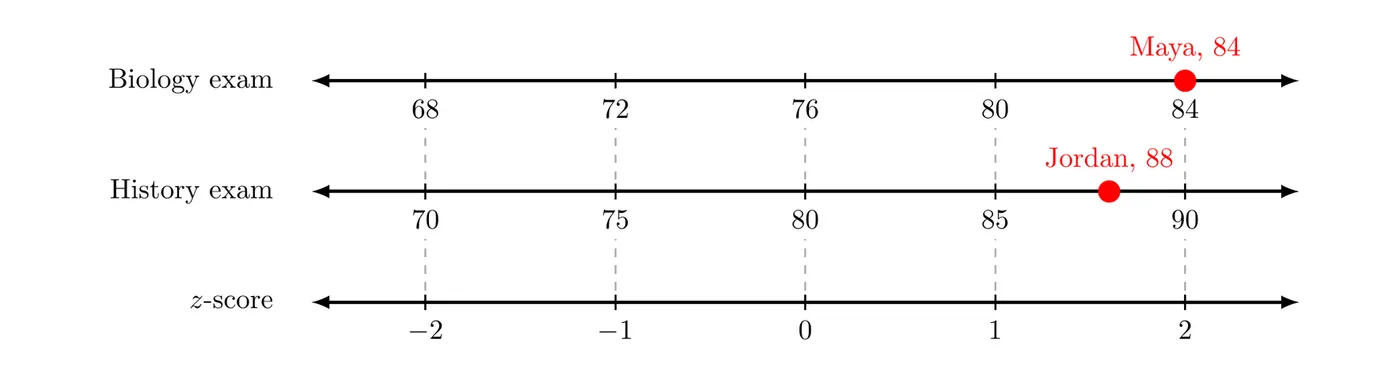
z_{\text{Maya}} = \frac{84 - 76}{4} = \frac{8}{4} = 2.0 \qquad z_{\text{Jordan}} = \frac{88 - 80}{5} = \frac{8}{5} = 1.6

Answer: Maya's score is 2.0 standard deviations above her class mean, while Jordan's is 1.6 standard deviations above his. Even though Jordan's raw score is higher, Maya did better relative to her class.

Example 6: When lower is better

In a 5K race, runners aged 16 to 17 had a mean time of 27.5 minutes with a standard deviation of 3.0 minutes. Runners aged 40 to 44 had a mean of 31.0 minutes with a standard deviation of 4.0 minutes. Sam (age 16) ran 22.4 minutes and Pat (age 42) ran 25.0 minutes. Relative to their age groups, who ran better?

z_{\text{Sam}} = \frac{22.4 - 27.5}{3.0} = \frac{-5.1}{3.0} = -1.7 \qquad z_{\text{Pat}} = \frac{25.0 - 31.0}{4.0} = \frac{-6.0}{4.0} = -1.5

Answer: Sam's time is 1.7 standard deviations below his group's mean, and Pat's is 1.5 standard deviations below hers. In a race, a lower time is better, so the more negative

z

-score wins: Sam ran better relative to his age group.

Common mistakes

Writing two separate descriptions without comparison words. Say which group is greater, smaller, or more variable.

Comparing only the centers. Cover shape, center, variability, and unusual features.

Putting graphs on different scales, which makes a comparison misleading.

Using boxplots to talk about clusters, gaps, or the number of peaks.

Interpreting $z = 2$ as "2 points above the mean." It means 2 standard deviations above the mean.

Forgetting which direction is better. With times or costs, a more negative $z$ -score is the better result.

Treating a difference between two samples as proof about the populations, or as proof of cause and effect.

Back Next