1.8 - Graphical Representations of Summary Statistics for One Quantitative Variable

Overview

A boxplot turns five summary statistics into a picture. It's quick to draw, it shows outliers clearly, and it makes comparing groups easy (you'll do that in Topic 1.9). This topic covers how to build a boxplot, including how to handle outliers, what a boxplot does and doesn't show, and how the mean and median reveal the shape of a distribution.

The five-number summary

The five-number summary is the minimum, the first quartile (

Q_1

), the median, the third quartile (

Q_3

), and the maximum. These five values split the ordered data into four parts with about 25% of the values in each.

Building a boxplot

A boxplot is a graph of the five-number summary:

The box goes from $Q_1$ to $Q_3$ , so it holds the middle 50% of the data. A line inside the box marks the median.

Lines called whiskers extend from the box out to the minimum and to the maximum. Each whisker represents about 25% of the data.

If there are outliers, each whisker stops at the most extreme data value that is not an outlier, and each outlier is marked separately, usually with an asterisk or a dot. A boxplot drawn this way is sometimes called a modified boxplot.

To build one:

Put the data in order and find the five-number summary.

Find the fences, $Q_1 - 1.5 \times \text{IQR}$ and $Q_3 + 1.5 \times \text{IQR}$ , and check for outliers.

Draw a number line with a scale, and label it with the variable and its units.

Draw the box from $Q_1$ to $Q_3$ with a line at the median.

Draw the whiskers to the most extreme values that are not outliers, then mark any outliers.

Example 1: Building a boxplot

A high school basketball player scored these points in 12 games: 8, 10, 11, 12, 12, 14, 15, 16, 18, 19, 21, 34. Make a boxplot.

Step 1: Five-number summary. There are 12 values, so the median is the mean of the 6th and 7th values, and each half has 6 values.

\text{median} = \frac{14 + 15}{2} = 14.5 \qquad Q_1 = \frac{11 + 12}{2} = 11.5 \qquad Q_3 = \frac{18 + 19}{2} = 18.5

The five-number summary is 8, 11.5, 14.5, 18.5, 34.

Step 2: Check for outliers.

\text{IQR} = 18.5 - 11.5 = 7 \qquad 1.5 \times 7 = 10.5

\text{lower fence} = 11.5 - 10.5 = 1 \qquad \text{upper fence} = 18.5 + 10.5 = 29

The 34-point game is above 29, so it's an outlier. Nothing is below 1.

Step 3: Whiskers. The left whisker goes to the minimum, 8. The right whisker stops at 21, the largest score that is not an outlier, and 34 gets its own symbol.

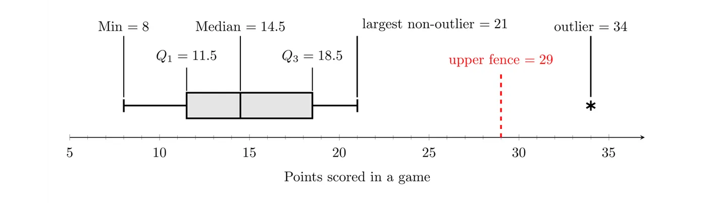
1.8 - Graphical Representations of Summary Statistics for One Quantitative Variable

Answer: The boxplot shows that the player's typical game was about 14.5 points, the middle half of the games ranged from 11.5 to 18.5 points, and the 34-point game was unusually high.

TI-84: enter the data in L1. Press 2nd then Y= (STAT PLOT), choose Plot1, turn it On, pick the boxplot icon that shows outliers as separate points (the modified boxplot), set Xlist to L1, then press ZOOM and choose 9:ZoomStat. Press TRACE to read the five-number summary.

Reading a boxplot

A boxplot shows the center (the median), the variability (the IQR is the length of the box and the range is the full width), outliers, and whether the distribution is skewed or symmetric.

Each of the four sections (left whisker, left part of the box, right part of the box, right whisker) holds about 25% of the data. So a longer section doesn't hold more data. It means the same 25% of the values are more spread out there.

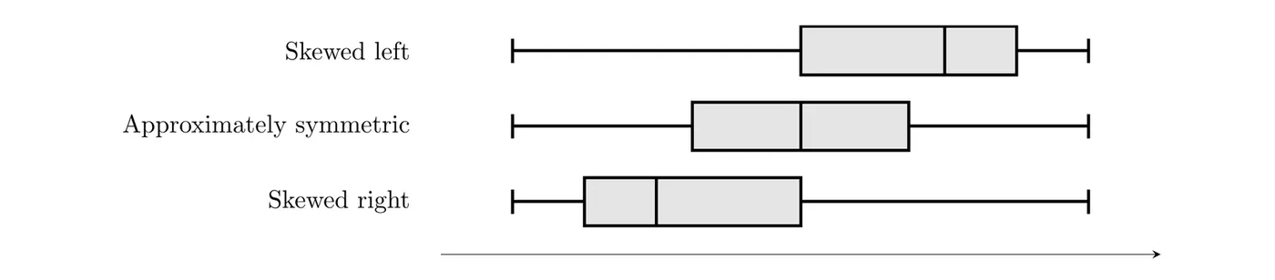
Skewed right: the median sits closer to $Q_1$ , and the right whisker is longer than the left.

Skewed left: the median sits closer to $Q_3$ , and the left whisker is longer than the right.

Approximately symmetric: the median is near the middle of the box, and the whiskers are about the same length.

What a boxplot hides

A boxplot shows only five numbers (plus any outliers), so it can't show individual values, the number of peaks, clusters, or gaps. It doesn't show the sample size either. Here are the geyser eruption times from Topic 1.6 as a dotplot and as a boxplot. The dotplot shows two clusters with a gap between them. The boxplot just looks skewed left.

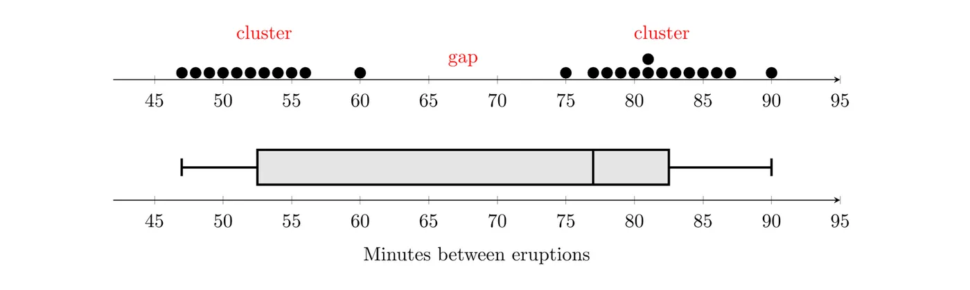
When the shape matters, look at a dotplot, stemplot, or histogram too.

The mean, the median, and shape

The mean is pulled toward a long tail, but the median isn't (the mean is nonresistant and the median is resistant). That gives a link between the two measures of center and the shape of the distribution:

Approximately symmetric: the mean and median are close to each other.

Skewed right: the mean is usually larger than the median, because the long right tail pulls the mean up.

Skewed left: the mean is usually smaller than the median, because the long left tail pulls the mean down.

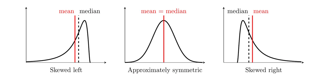
Notice the word "usually." This pattern holds for most real data, but there are exceptions, especially with discrete data or several peaks. Treat it as evidence about shape, not proof. It also works in reverse: a mean much larger than the median suggests a right skew or high outliers.

Example 2: What the mean and median say about shape

At a tech company, the mean salary is $82,000 and the median salary is $61,000. What does this suggest about the distribution of salaries?

Answer: The mean is much larger than the median, so the distribution of salaries is probably skewed right: most employees earn moderate salaries, and a few very high salaries pull the mean up. The median, $61,000, better describes what a typical employee earns.

Example 3: Reading a boxplot (AP-style)

The boxplot summarizes the lengths of 200 songs on a playlist.

(a) Give the five-number summary and identify any outliers. (b) Is the mean song length more likely to be greater than or less than the median? Explain. (c) About how many songs are longer than 4.2 minutes?

(a) Reading the plot: minimum 2.0,

Q_1 = 3.0

, median 3.4,

Q_3 = 4.2

, and maximum 6.9 minutes. The two songs marked with asterisks, at about 6.3 and 6.9 minutes, are outliers. Check with the fences:

\text{IQR} = 4.2 - 3.0 = 1.2 \qquad 1.5 \times 1.2 = 1.8

\text{upper fence} = 4.2 + 1.8 = 6.0 \qquad \text{lower fence} = 3.0 - 1.8 = 1.2

Both 6.3 and 6.9 are above 6.0, and the right whisker ends at 5.7 minutes, the longest song that isn't an outlier. No song is below 1.2 minutes.

(b) The distribution is skewed right. The median (3.4) is closer to

Q_1

(0.4 minutes away) than to

Q_3

(0.8 minutes away), the right whisker (4.2 to 5.7, 1.5 minutes long) is longer than the left whisker (2.0 to 3.0, 1.0 minute long), and both outliers are on the high end. A right skew pulls the mean up, so the mean song length is most likely greater than the median of 3.4 minutes.

(c) About 25% of the songs are longer than

Q_3 = 4.2

minutes, and 25% of 200 is 50, so about 50 songs are longer than 4.2 minutes.

Common mistakes

Drawing a whisker all the way to an outlier. Whiskers stop at the most extreme value that isn't an outlier.

Thinking a longer section of a boxplot holds more data. Every section holds about 25%.

Using a boxplot to talk about peaks, clusters, or gaps. A boxplot can't show them.

Leaving the number line without a scale or a label with units.

Saying the mean is always larger than the median in a skewed right distribution. It's usual, not guaranteed.

Reading meaning into how tall the box is drawn. Only lengths along the number line matter.

Back Next