4.2 - Constructing a Confidence Interval for a Population Mean or Population Mean Difference

Overview

In real studies you almost never know the population standard deviation

\sigma

, so an interval for a mean uses the sample standard deviation

s

and a

t

-distribution. This topic covers

t

-distributions, the one-sample

t

-interval for a population mean

\mu

, and the same interval for a population mean difference

\mu_d

in a matched pairs design.

Why not just use $z$ ?

In Topic 4.1,

z = \frac{\bar{x} - \mu}{\sigma/\sqrt{n}}

had a standard normal distribution. When

\sigma

is unknown, you replace it with

s

t = \frac{\bar{x} - \mu}{s / \sqrt{n}}

This statistic varies more than

z

does, because now two things change from sample to sample:

\bar{x}

and

s

, and small samples give especially shaky values of

s

. So the distribution of

t

has more area in its tails than the standard normal, and using

z^*

would make intervals that are too narrow. The rule: use a

t

-distribution for critical values and test statistics whenever

\sigma

is unknown and

s

is used in its place, which is nearly always.

Describing $t$ -distributions

The

t

-distributions (also called Student's

t

-distributions) are a family of curves:

Shape: each one is symmetric, bell-shaped, and centered at 0, like the standard normal curve. They're standardized distributions.

Degrees of freedom: a specific $t$ -distribution is identified by its degrees of freedom (df), which are based on the sample size. For one sample of size $n$ , $\text{df} = n - 1$ .

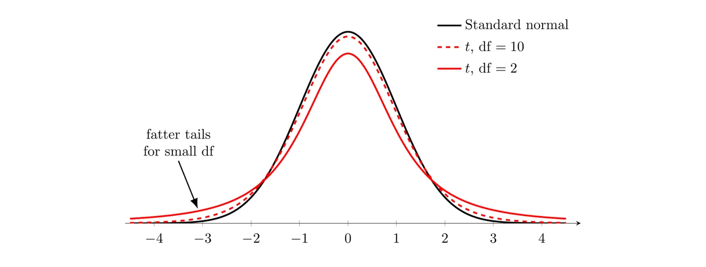
Tails: when df is small, the $t$ -distribution has a lower peak and fatter tails than the standard normal: less of its area sits near 0 and more sits far out in the tails. That makes it more spread out.

Large df: as df increases, the $t$ -distribution looks more and more like the standard normal distribution (mean 0, standard deviation 1). With very large df they're nearly identical.

4.2 - Constructing a Confidence Interval for a Population Mean or Population Mean Difference

Critical values

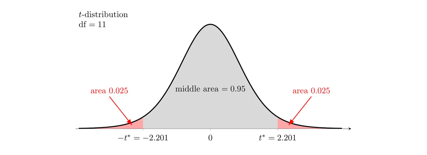
For a C% confidence interval,

t^*

is the value that puts the middle C% of the

t

-distribution with

n - 1

degrees of freedom between

-t^*

and

t^*

. Here is

t^*

for 95% confidence with df = 11:

Table B: use the row for your df and the column for your confidence level C (along the bottom). If your df isn't in the table, use the next smaller df, which gives a slightly larger $t^*$ and a slightly wider, more cautious interval.

TI-84: invT(area to the left, df). For 95% confidence with df = 11, invT(0.975, 11) gives 2.201.

As df grows,

t^*

shrinks toward

z^* = 1.960

df	2	5	11	30	100	$\infty$ (this is $z^*$ )
$t^*$ for 95% confidence	4.303	2.571	2.201	2.042	1.984	1.960

Choosing the procedure and the parameter

One sample

To estimate the population mean of a quantitative variable from one sample, use a one-sample

t

-interval for a population mean.

Matched pairs

In a matched pairs design, the two samples are dependent: each value in one group is linked to one specific value in the other, like the same person measured before and after, or twins split between two treatments. Don't treat the two columns as separate samples. Subtract within each pair to get one sample of differences, then use a one-sample

t

-interval for a population mean difference

\mu_d

(often called a paired

t

-interval).

Stating the parameter

Define the parameter in words, in context: the population mean or mean difference, the response variable, and the population. For example,

\mu

= the true mean caffeine content (mg) of all large cold brews sold by the chain. For a mean difference

\mu_d

, always state the order of subtraction (like after minus before). It decides what a positive or negative value means.

Conditions

A one-sample

t

-interval for

\mu

\mu_d

requires three conditions:

Randomization condition: the data should be collected using a random sample or a randomized experiment.

10% condition: when sampling without replacement, the population size must be at least 10 times the sample size, $n \le 10\%N$ . This keeps the observations close enough to independent.

Sample data condition (some books call it the normal/large sample condition). At least one of these is true:

the problem says the population distribution is approximately normal, or

$n \ge 30$ , or

$n < 30$ and a graph of the sample data (dotplot, boxplot, or stemplot) shows no strong skewness and no outliers.

For matched pairs, check everything on the differences: the number of differences should be at least 30, or the sample of differences should be free from strong skewness and outliers.

When

n < 30

, actually make the graph (or describe it) in your answer. Writing "the data look normal" with no evidence doesn't earn credit.

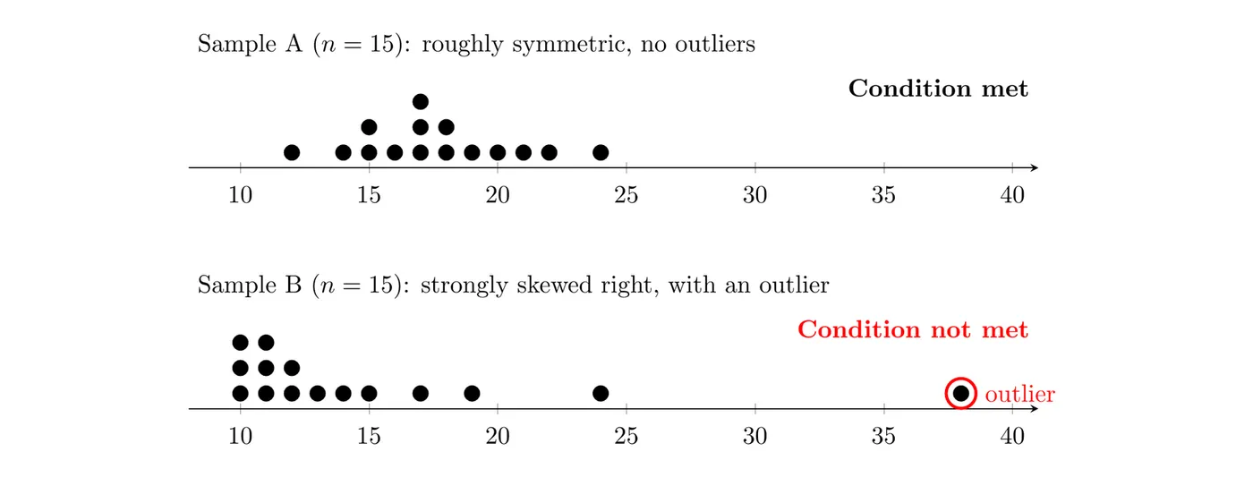
Why it matters:

t

procedures assume the sampling distribution of

\bar{x}

is approximately normal, and with a small sample the data are your only clue to the population's shape. An outlier also drags

\bar{x}

and inflates

s

Calculating the interval

The point estimate for

\mu

is the sample mean

\bar{x}

. For

\mu_d

, it's the mean of the sample differences,

\bar{x}_d

The standard error of

\bar{x}

estimates how far

\bar{x}

typically falls from

\mu

SE_{\bar{x}} = \frac{s}{\sqrt{n}}

The margin of error (MOE) is the critical value times the standard error, and the interval is the point estimate plus or minus the margin of error:

\text{MOE} = t^* \left( \frac{s}{\sqrt{n}} \right) \qquad\qquad \bar{x} \pm t^* \frac{s}{\sqrt{n}}, \quad \text{df} = n - 1

This is the formula sheet's general form, statistic ± (critical value)(standard error of the statistic). For matched pairs, use

\bar{x}_d

s_d

, and

n

= the number of pairs.

TI-84: STAT, TESTS, 8:TInterval (Data for a list, Stats for

\bar{x}

s

, and

n

; for matched pairs, put the differences in a list first). On the AP exam, still name the procedure and show the formula with numbers.

Example 1: Caffeine in cold brew

A consumer group wants to estimate the mean caffeine content of a coffee chain's large cold brew. They buy one large cold brew at each of 12 randomly selected locations and measure the caffeine (mg):

188, 195, 201, 204, 207, 210, 213, 215, 219, 224, 228, 240

Construct and interpret a 95% confidence interval for the mean caffeine content of all large cold brews sold by this chain.

State: We want to estimate

\mu

= the true mean caffeine content (mg) of all large cold brews sold by this chain, with 95% confidence.

Plan: One-sample

t

-interval for a population mean. Check the conditions:

Randomization: the drinks came from 12 randomly selected locations.

10%: 12 drinks is far less than 10% of all the large cold brews this chain sells.

Sample data: $n = 12 < 30$ , so graph the data. The dotplot is roughly symmetric with no outliers, so a $t$ procedure is reasonable.

Do: From the data,

\bar{x} = 212.0

mg and

s \approx 14.53

mg. With

\text{df} = 12 - 1 = 11

t^* = 2.201

SE_{\bar{x}} = \frac{14.53}{\sqrt{12}} \approx 4.194 \qquad \text{MOE} = 2.201(4.194) \approx 9.23

212.0 \pm 9.23 = (202.8, \; 221.2)

Conclude: We are 95% confident that the interval from 202.8 mg to 221.2 mg captures the true mean caffeine content of all large cold brews sold by this chain.

Example 2: A reading program (matched pairs)

A school district randomly selects 10 of the 300 students in its summer reading program. Each student's reading score (words read correctly per minute) is measured at the start and at the end of the program.

Student	Before	After	Difference (after minus before)
1	92	95	3
2	105	114	9
3	78	83	5
4	118	116	$-2$
5	96	104	8
6	84	90	6
7	110	121	11
8	99	103	4
9	88	95	7
10	101	110	9

Construct and interpret a 95% confidence interval for the mean change in reading score.

State:

\mu_d

= the true mean difference in reading score (after minus before, in words per minute) for all students in the summer program. We'll estimate it with 95% confidence.

Plan: The before and after scores come from the same students, so the data are paired. Use a one-sample

t

-interval for a population mean difference.

Randomization: the 10 students were randomly selected.

10%: $10 \le 10\%(300) = 30$ .

Sample data: there are only 10 differences, so graph them. The dotplot shows no strong skewness and no outliers. The value $-2$ sits a little apart, but with $Q_1 = 4$ and $Q_3 = 9$ the lower fence is $4 - 1.5(5) = -3.5$ , and $-2$ is inside it.

Do: For the 10 differences,

\bar{x}_d = 6.0

and

s_d \approx 3.74

. With df = 9,

t^* = 2.262

SE = \frac{3.74}{\sqrt{10}} \approx 1.183 \qquad \text{MOE} = 2.262(1.183) \approx 2.68

6.0 \pm 2.68 = (3.32, \; 8.68)

Conclude: We are 95% confident that the interval from 3.32 to 8.68 words per minute captures the true mean difference in reading score (after minus before) for all students in this summer program. Because the order is after minus before, positive values mean scores went up.

Example 3: Summary statistics only (AP-style)

A hospital randomly selects 50 of last month's 900 emergency room visits and records each patient's wait time. The sample mean is 47.3 minutes and the sample standard deviation is 21.8 minutes. A dotplot of the 50 wait times is skewed to the right. Construct and interpret a 90% confidence interval for the mean wait time of all ER visits last month.

State:

\mu

= the true mean ER wait time (minutes) for all 900 visits last month, estimated with 90% confidence.

Plan: One-sample

t

-interval for a population mean. Randomization: the visits were randomly selected. 10%:

50 \le 10\%(900) = 90

. Sample data: the sample is skewed, but

n = 50 \ge 30

, so the sampling distribution of

\bar{x}

is approximately normal by the central limit theorem.

Do: df = 49. Technology gives invT(0.95, 49) = 1.677. (Table B's df = 40 row gives

t^* = 1.684

, slightly more conservative.)

SE_{\bar{x}} = \frac{21.8}{\sqrt{50}} \approx 3.083 \qquad \text{MOE} = 1.677(3.083) \approx 5.17

47.3 \pm 5.17 = (42.1, \; 52.5)

Conclude: We are 90% confident that the interval from 42.1 to 52.5 minutes captures the true mean wait time for all ER visits at this hospital last month.

Common mistakes

Using $z^*$ instead of $t^*$ for a mean when $\sigma$ is unknown.

Using the wrong df. For one sample or matched pairs, df = $n - 1$ , where $n$ is the number of individuals or pairs.

Treating paired data as two independent samples. If each value in one group is linked to one value in the other, work with the differences.

Leaving out the order of subtraction for $\mu_d$ , or describing the parameter as a sample statistic ("the mean of these 10 students").

Saying the data are normal with no evidence. For $n < 30$ , show or describe a graph of the sample data (or of the differences).

Back Next