4.5 - Carrying Out a Test for a Population Mean or Population Mean Difference

Overview

Once a test is set up (Topic 4.4), you carry it out: compute the

t

test statistic, find the

p

-value, compare the

p

-value to the significance level, and state a conclusion in context. This page finishes the bottle and caffeine tests from Topic 4.4 and shows how to read computer output.

The test statistic

t = \frac{\bar{x} - \mu_0}{s / \sqrt{n}}, \qquad \text{df} = n - 1

This is the formula sheet's standardized test statistic: (statistic minus parameter) divided by (standard error of the statistic). The numerator is how far the sample mean is from the null value. The denominator is how far

\bar{x}

typically falls from

\mu

just by chance. So

t

counts how many standard errors

\bar{x}

is from

\mu_0

For matched pairs, use the differences:

t = \frac{\bar{x}_d - 0}{s_d/\sqrt{n}}

, where

n

is the number of pairs.

When the null hypothesis is true (and the conditions are met), this statistic has a

t

-distribution with

n - 1

degrees of freedom. That's the distribution you use to find the

p

-value.

Finding the $p$ -value

The

p

-value is the probability of getting a test statistic as extreme as the one observed, or more extreme, in the direction of the alternative hypothesis, assuming the null hypothesis is true. It's an area under the

t

-curve with

n - 1

df:

Alternative hypothesis	$p$ -value
$H_a: \mu < \mu_0$	Area to the left of $t$
$H_a: \mu > \mu_0$	Area to the right of $t$
$H_a: \mu \ne \mu_0$	Twice the area beyond $\|t\|$ (both tails)

Technology: on a TI-84, tcdf(lower, upper, df) gives an area, for example tcdf(-1E99, -2.64, 24). Or run STAT, TESTS, 2:T-Test, which reports $t$ , the $p$ -value, $\bar{x}$ , $s$ , and $n$ .

Table B: in your df row, find the two critical values that $|t|$ falls between. The tail probabilities at the top of those columns bound the $p$ -value. For a two-sided test, double them.

Interpreting the $p$ -value

An interpretation must say that the

p

-value was computed assuming the null hypothesis is true, with the null value in context. A template:

Assuming the true mean [context] is [null value], there is about a [ $p$ -value] probability of getting a sample mean of [observed value] or [more extreme, in the direction of the alternative], just by chance.

A small

p

-value means the observed result would rarely happen if

H_0

were true, so it's evidence for

H_a

. A

p

-value that isn't small means the result is the kind of thing that happens by chance when

H_0

is true, so it isn't convincing evidence for

H_a

. It also isn't evidence that

H_0

is true.

Making a decision and a conclusion

A formal decision compares the

p

-value to the significance level

\alpha

(given in the problem, or chosen before the study):

If $p$ -value $\le \alpha$ : reject $H_0$ . There is convincing statistical evidence for $H_a$ .

If $p$ -value $> \alpha$ : fail to reject $H_0$ . There is not convincing statistical evidence for $H_a$ .

Then write the conclusion in context. It should:

compare the $p$ -value to $\alpha$ explicitly ("Because the $p$ -value of 0.007 is less than $\alpha = 0.05$ ..."),

be stated in terms of the alternative hypothesis,

refer to the parameter and the population, and

use non-definitive language: "there is convincing evidence that..." Never write "this proves" or "accept $H_0$ ."

The conclusion is the statistical answer to the investigative question that started the study (is the machine underfilling? does caffeine change reaction time?).

Example 1: Are bottles underfilled? (finishing the test)

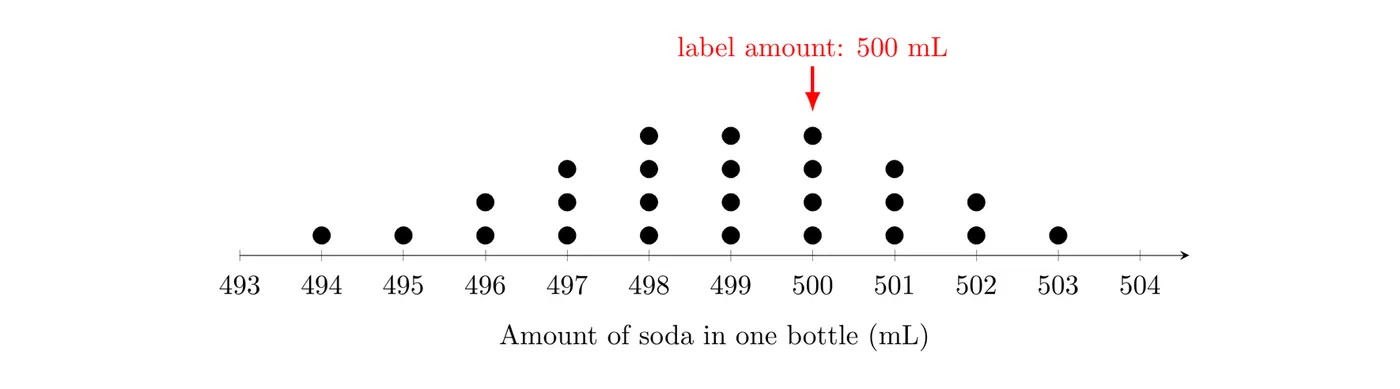
From Topic 4.4: an inspector randomly selects 25 of the 8,000 bottles a machine filled today to test whether the machine underfills. The sample mean is

\bar{x} = 498.8

mL and the sample standard deviation is

s \approx 2.27

mL. Use

\alpha = 0.05

State:

H_0: \mu = 500

and

H_a: \mu < 500

, where

\mu

is the true mean amount of soda (mL) in all bottles filled by this machine today. Use

\alpha = 0.05

Plan: One-sample

t

-test for a population mean. Randomization: the 25 bottles were a random sample. 10%:

25 \le 10\%(8{,}000) = 800

. Sample data:

n = 25 < 30

, but the dotplot is roughly symmetric with no outliers.

4.5 - Carrying Out a Test for a Population Mean or Population Mean Difference

Do:

t = \frac{498.8 - 500}{2.27 / \sqrt{25}} = \frac{-1.2}{0.454} \approx -2.64, \qquad \text{df} = 24

The

p

-value is the area to the left of

t = -2.64

under the

t

-distribution with 24 df, which is about 0.007 (tcdf(-1E99, -2.64, 24)). With Table B, 2.64 falls between 2.492 (tail probability 0.01) and 2.797 (tail probability 0.005), so the

p

-value is between 0.005 and 0.01.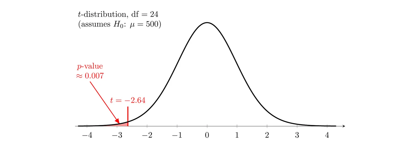

Interpret the

p

-value: Assuming the true mean amount of soda in today's bottles is 500 mL, there is about a 0.007 probability of getting a sample mean of 498.8 mL or less in a random sample of 25 bottles, just by chance.

Conclude: Because the

p

-value of 0.007 is less than

\alpha = 0.05

, we reject

H_0

. There is convincing statistical evidence that the true mean amount of soda in all bottles filled by this machine today is less than 500 mL.

Example 2: Caffeine and reaction time (finishing the test)

From Topic 4.4: 14 volunteers each took a reaction-time test after a caffeine pill and after a placebo, in random order. For the 14 differences (caffeine minus placebo),

\bar{x}_d \approx -9.29

ms and

s_d \approx 13.90

ms. Test at

\alpha = 0.05

whether caffeine changes mean reaction time.

State:

H_0: \mu_d = 0

and

H_a: \mu_d \ne 0

, where

\mu_d

is the true mean difference in reaction time (caffeine minus placebo, in ms) for adults like these volunteers. Use

\alpha = 0.05

Plan: One-sample

t

-test for a population mean difference (paired). Randomization: the order of the pills was randomly assigned. 10%: doesn't apply to an experiment. Sample data: the dotplot of the 14 differences is roughly symmetric with no outliers.

Do:

t = \frac{-9.29 - 0}{13.90 / \sqrt{14}} = \frac{-9.29}{3.71} \approx -2.50, \qquad \text{df} = 13

The alternative is two-sided, so the

p

-value is the area beyond 2.50 in both tails. Each tail has area about 0.0133, so the

p

-value is about

2(0.0133) = 0.0266

. With Table B (df = 13), 2.50 falls between 2.282 (tail probability 0.02) and 2.650 (tail probability 0.01), so one tail is between 0.01 and 0.02 and the two-sided

p

-value is between 0.02 and 0.04.

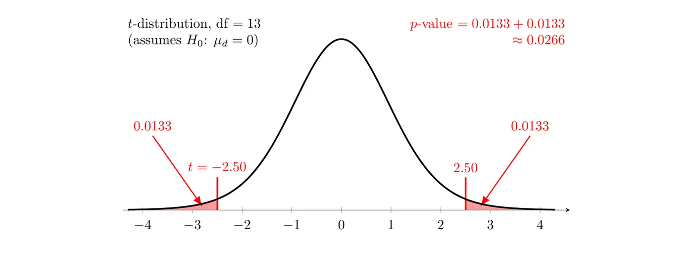
Interpret the

p

-value: Assuming caffeine has no effect on the mean reaction time of adults like these (

\mu_d = 0

), there is about a 0.027 probability of getting a mean difference at least 9.29 ms away from 0, in either direction, just by chance.

Conclude: Because the

p

-value of 0.027 is less than

\alpha = 0.05

, we reject

H_0

. There is convincing statistical evidence that caffeine changes the true mean reaction time for adults like these volunteers. The sample mean difference is negative, so the data suggest caffeine lowers (speeds up) reaction time, and because the order of the pills was randomly assigned, we can attribute the difference to the caffeine.

Two side notes. At

\alpha = 0.01

, the same

p

-value would lead to failing to reject

H_0

, which is why

\alpha

is set before the data are analyzed. And a 95% confidence interval for

\mu_d

-9.29 \pm 2.160(3.71) = (-17.3, -1.3)

ms, doesn't contain 0, which agrees with rejecting

H_0

in a two-sided test at

\alpha = 0.05

Example 3: Reading computer output (AP-style)

A researcher wonders whether students at a large high school (2,100 students) average more than 7 hours of screen time per day. She takes a random sample of 35 students. A dotplot of their screen times is moderately skewed to the right with no outliers. Software gives this output for

H_0: \mu = 7

and

H_a: \mu > 7

, where

\mu

is the true mean daily screen time (hours) for all students at the school:

Variable	N	Mean	StDev	SE Mean	T	P
Screen time (hours)	35	7.42	1.96	0.331	1.27	0.107

(a) Are the conditions met? (b) Interpret the

p

-value. (c) What should she conclude at

\alpha = 0.05

(a) Yes. Randomization: random sample of students. 10%:

35 \le 10\%(2{,}100) = 210

. Sample data: the data are skewed, but

n = 35 \ge 30

, so the sampling distribution of

\bar{x}

is approximately normal.

(b) The output's test statistic is

t = \frac{7.42 - 7}{0.331} \approx 1.27

with df = 34, and the

p

-value is 0.107. Assuming the true mean daily screen time for students at this school is 7 hours, there is about a 0.107 probability of getting a sample mean of 7.42 hours or more in a random sample of 35 students, just by chance.

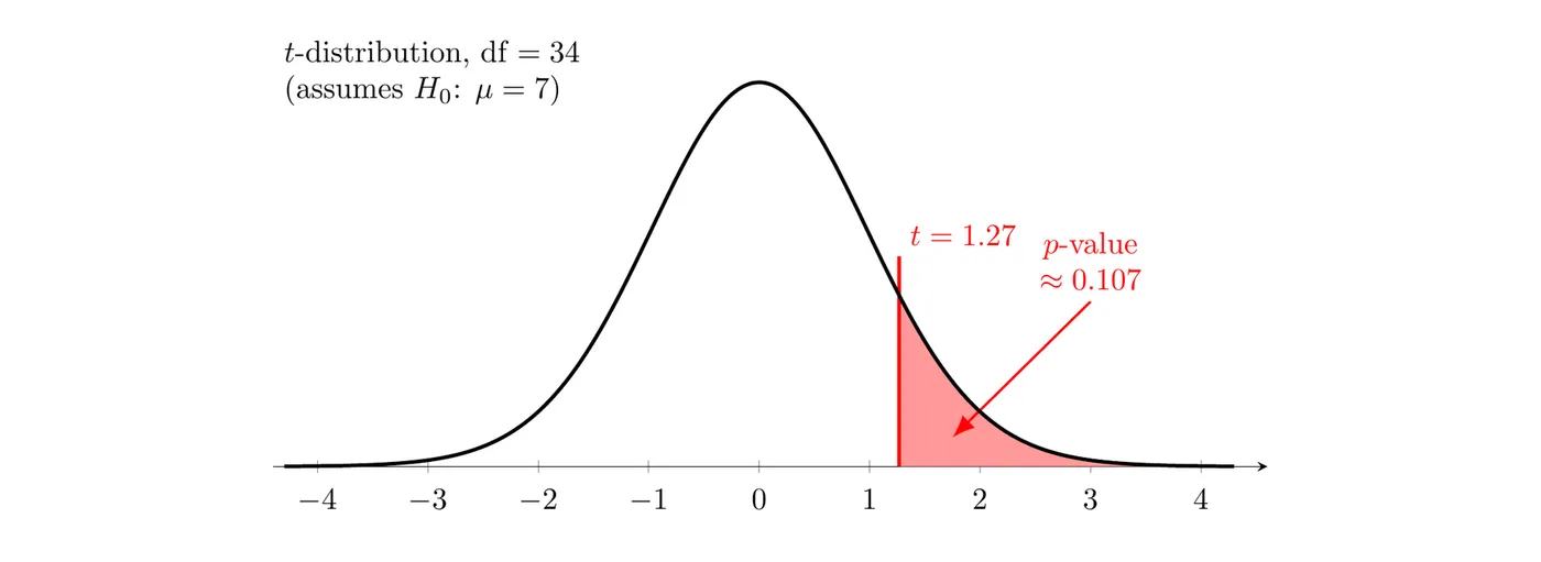
(c) Because the

p

-value of 0.107 is greater than

\alpha = 0.05

, we fail to reject

H_0

. There is not convincing statistical evidence that the true mean daily screen time for students at this school is more than 7 hours.

This does not show the mean is exactly 7 hours. A sample mean of 7.42 hours happens fairly often by chance when

\mu = 7

, so the data just aren't strong enough to rule 7 out.

Errors to keep in mind

Any decision from a test can be wrong, and Topic 3.8 covers both errors in full. Example 1 rejected

H_0

, so the only possible error there is a Type I error: concluding the machine underfills when its true mean really is 500 mL. Example 3 failed to reject

H_0

, so the only possible error is a Type II error: missing that the true mean screen time really is above 7 hours.

Common mistakes

Using normalcdf or Table A for a $t$ statistic, or using the wrong df.

Forgetting to double the tail area for a two-sided alternative.

Interpreting the $p$ -value as the probability that $H_0$ is true. It's computed by assuming $H_0$ is true.

Concluding without comparing the $p$ -value to $\alpha$ , or writing "accept $H_0$ " or "proves."

Stopping at "reject $H_0$ " with no context, parameter, or population.

For paired data, running a two-sample test, or mixing up the order of subtraction when reading the sign of $t$ .

Back Next

4.5 - Carrying Out a Test for a Population Mean or Population Mean Difference

Overview

The test statistic

Finding the ppp-value

Interpreting the ppp-value

Making a decision and a conclusion

Example 1: Are bottles underfilled? (finishing the test)

Example 2: Caffeine and reaction time (finishing the test)

Example 3: Reading computer output (AP-style)

Errors to keep in mind

Common mistakes

Finding the $p$ -value

Interpreting the $p$ -value