4.8 - Justifying a Claim Based on a Confidence Interval for the Difference Between Two Population Means

Overview

Once you have a confidence interval for

\mu_1 - \mu_2

, you need to say what it means and what it lets you conclude. This topic covers what AP graders look for: interpreting the interval, interpreting the confidence level, and using the interval to support or refute a claim about the difference in population means, especially by checking whether the interval contains 0.

An interval can miss

A confidence interval for the difference between two population means is calculated from samples of two populations, and samples vary. A different pair of samples would give a different

\bar{x}_1 - \bar{x}_2

and a different interval. So any single interval may or may not contain the true value of

\mu_1 - \mu_2

, and you never know for sure whether yours does. That's why the language is "confident," not "certain."

What the confidence level means

The confidence level describes the method, not one interval: in repeated random sampling with the same sample sizes from the same populations, about C% of the intervals created will capture the difference between the two population means.

The figure shows a simulation where the truth is known. Two normal populations have means that differ by exactly 5, so

\mu_1 - \mu_2 = 5

. Forty pairs of random samples (

n_1 = n_2 = 30

) each produced a 95% two-sample

t

-interval. 38 of the 40 intervals (95%) capture 5; the two in red miss.

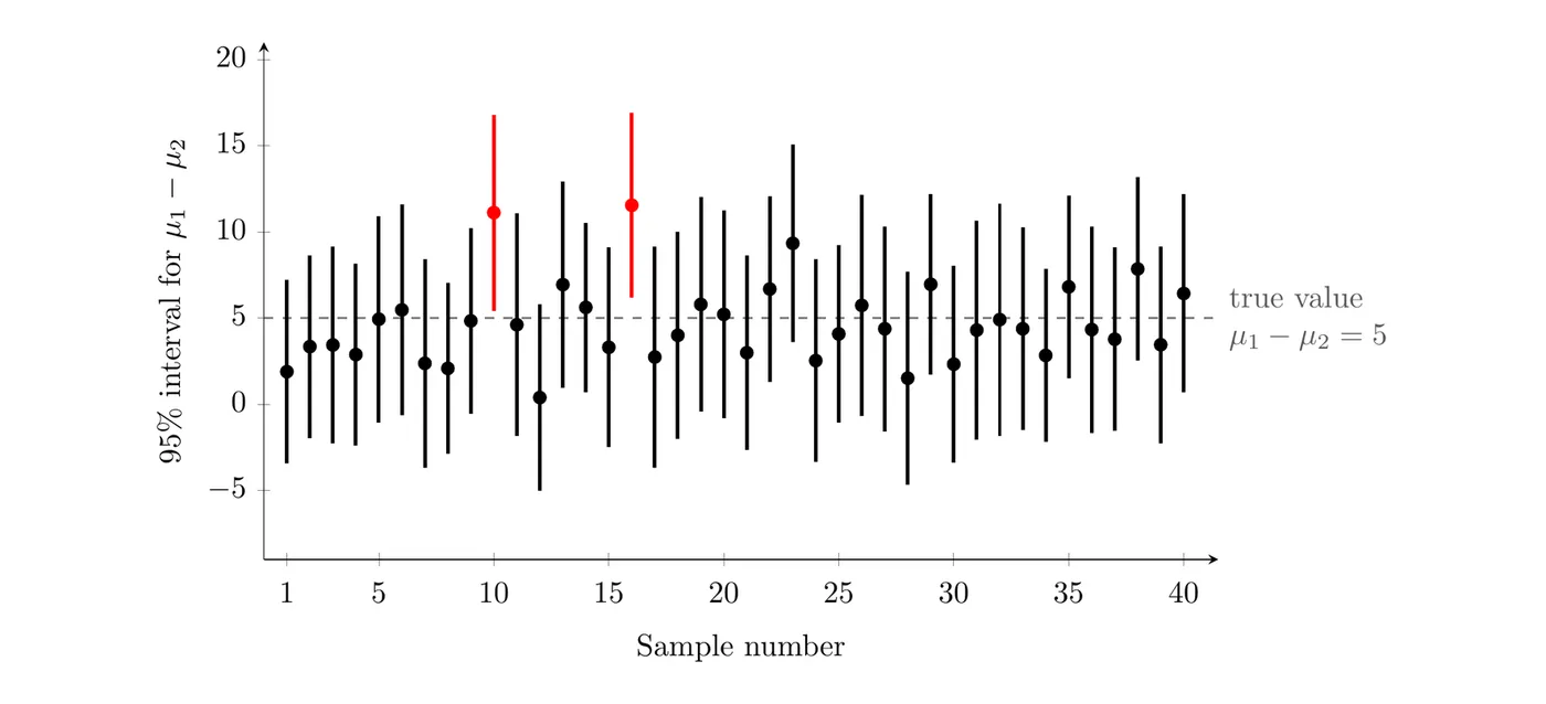
4.8 - Justifying a Claim Based on a Confidence Interval for the Difference Between Two Population Means

Every interval in the picture was made the same way. The red ones are the bad luck the 95% allows for. With real data you get only one interval, and you can't tell which kind it is.

Template: If we took many pairs of random samples of these sizes from [population 1] and [population 2] and built a C% confidence interval from each pair, about C% of those intervals would capture the true difference in mean [variable].

Interpreting the interval

To interpret a specific C% interval

(a, b)

, say you're C% confident that it captures the true difference in population means, with the variable, the populations, and the order of subtraction in context:

We are C% confident that the interval from $a$ to $b$ captures the true difference in mean [response variable] ([population 1] minus [population 2]).

AP scoring looks for three things: the confidence level, the endpoints, and context that names the parameter (the difference in true means, the variable, and both populations). Compare these attempts for the pizza delivery interval in Example 2:

Interpretation	Verdict
We are 90% confident that the interval from $-6.20$ to $-1.40$ minutes captures the true difference in mean delivery time (FastSlice minus PieDash) for all delivery orders from these two restaurants that month.	Complete
The interval is $(-6.20, -1.40)$ .	No confidence level, no context
We are 90% confident the true mean difference is between $-6.20$ and $-1.40$ .	Missing the variable, the populations, and the order
We are 90% confident that the difference in sample means is between $-6.20$ and $-1.40$ .	Wrong: the sample difference is known exactly ( $-3.8$ ). The interval is about the population means.
There is a 90% probability that $\mu_F - \mu_P$ is between $-6.20$ and $-1.40$ .	Wrong: $\mu_F - \mu_P$ is a fixed number. It's either in this interval or not.

Using the interval to judge a claim

A confidence interval gives a range of plausible values for

\mu_1 - \mu_2

, and that range can serve as evidence for or against a claim. The key value is 0, because

\mu_1 - \mu_2 = 0

means the two population means are equal.

The interval contains 0: a difference of 0 is plausible, so there is insufficient evidence to conclude there's a difference between the two population means. This doesn't prove the means are equal; it just isn't evidence that they differ.

The interval is entirely above 0: every plausible difference is positive, so there is convincing evidence that $\mu_1 > \mu_2$ .

The interval is entirely below 0: there is convincing evidence that $\mu_1 < \mu_2$ .

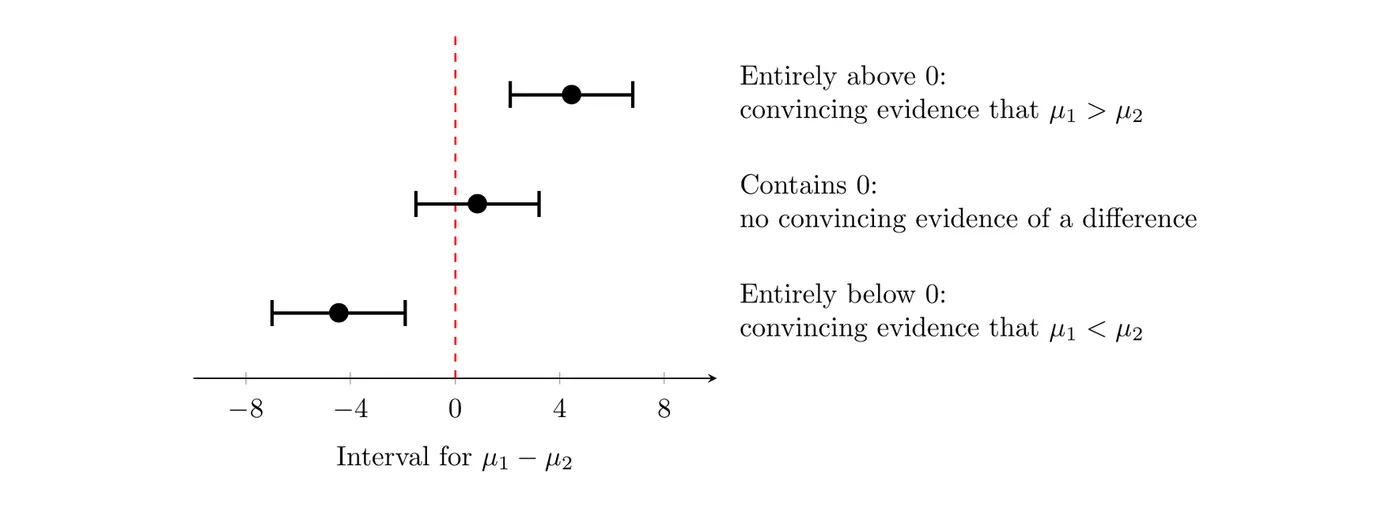
The same logic works for any claimed value. If someone claims the difference is at least 2, check whether every value in the interval is at least 2. If the claimed value sits inside the interval, it's plausible, but the data don't prove it.

On the exam, back up the decision with the interval: "Yes, because 0 is not in the interval

(-6.20, -1.40)

." The reasoning has to mention whether 0 (or the claimed value) is in the interval. A C% interval also lines up with a two-sided test at

\alpha = 1 - \frac{C}{100}

: if 0 is outside a 95% interval, a two-sided test at

\alpha = 0.05

would reject

H_0\colon \mu_1 = \mu_2

(Topics 4.9 and 4.10).

Example 1: Sleep for juniors and seniors

In Topic 4.7, Example 1, a 95% confidence interval for

\mu_J - \mu_S

came out to

(-0.10, 1.10)

hours, where

\mu_J

and

\mu_S

are the true mean hours of sleep on a school night for all juniors and all seniors at one large high school.

Interpret the interval.

A counselor claims that juniors at the school get more sleep than seniors, on average. Do the data support the claim?

Part 1. We are 95% confident that the interval from

-0.10

1.10

hours captures the true difference in mean hours of sleep on a school night (juniors minus seniors) for all juniors and seniors at this school.

Part 2. No. The interval contains 0, so equal means are plausible. The data don't give convincing evidence that juniors at this school get more sleep on average than seniors, even though the juniors in the sample averaged 0.5 hours more. The plausible values range from seniors sleeping 0.10 hours more to juniors sleeping 1.10 hours more.

Example 2: Pizza delivery times (AP-style)

A food writer takes a random sample of 60 delivery orders from FastSlice and an independent random sample of 50 delivery orders from PieDash during one month. FastSlice:

\bar{x}_F = 31.4

minutes,

s_F = 6.8

minutes. PieDash:

\bar{x}_P = 35.2

minutes,

s_P = 8.1

minutes. Each restaurant made thousands of deliveries that month.

Calculate a 90% two-sample $t$ -interval for $\mu_F - \mu_P$ , the difference in the true mean delivery times.

Interpret the interval.

Interpret the confidence level.

PieDash advertises that its deliveries are just as fast as FastSlice's, on average. Is there convincing statistical evidence of a difference in the true mean delivery times?

Part 1. Conditions: two independent random samples; 60 and 50 are each less than 10% of the thousands of deliveries; and both samples have at least 30 orders. Technology gives df

\approx 95.97

and

t^* \approx 1.661

(31.4 - 35.2) \pm 1.661\sqrt{\frac{6.8^2}{60} + \frac{8.1^2}{50}} = -3.8 \pm 1.661(1.443) = -3.8 \pm 2.40 = (-6.20,\ -1.40)

Part 2. We are 90% confident that the interval from

-6.20

-1.40

minutes captures the true difference in mean delivery time (FastSlice minus PieDash) for all delivery orders from these two restaurants that month.

Part 3. If we took many pairs of random samples (60 FastSlice orders and 50 PieDash orders) and built a 90% interval from each pair, about 90% of those intervals would capture the true difference in mean delivery time.

Part 4. Yes. Every value in the interval is negative, so 0 is not in the interval

(-6.20, -1.40)

. There is convincing evidence that the true mean delivery times differ. In fact, the interval suggests FastSlice's true mean delivery time is shorter than PieDash's by somewhere between 1.40 and 6.20 minutes, so the data contradict PieDash's ad.

Example 3: Judging a specific claim

Engineers randomly assign 70 phones to get either a new battery design or the old design, 35 phones each. New design:

\bar{x} = 14.6

hours,

s = 2.1

hours. Old design:

\bar{x} = 12.4

hours,

s = 2.5

hours. A 95% two-sample

t

-interval for

\mu_{\text{new}} - \mu_{\text{old}}

, the true difference in mean battery life (new minus old), is

(1.10, 3.30)

hours. The company wants to advertise that the new design lasts at least 2 hours longer on average. Is that claim supported?

Answer: Partly. The interval is entirely above 0, so there's convincing evidence that the new design lasts longer on average, and because the designs were randomly assigned, the new design is the likely cause. But the interval also contains values below 2, such as 1.5 hours, so a true difference smaller than 2 hours is plausible. The data don't give convincing evidence for the "at least 2 hours longer" claim. The company can claim the new battery lasts longer, but not by at least 2 hours.

Common mistakes

Treating the confidence level as a probability about one interval. The 95% describes the method over many samples.

Interpreting the interval as being about sample means or individual values. It estimates the difference in population means.

Leaving out the context (the variable, both populations, and the order of subtraction).

Saying an interval that contains 0 proves the means are equal. It only means there isn't convincing evidence of a difference.

Deciding without the interval. "The sample means are different, so the population means are different" ignores sampling variability. Base the decision on whether 0 is in the interval.

Back Next