4.4 - Setting Up a Test for a Population Mean or Population Mean Difference

Overview

A confidence interval estimates a mean. A significance test checks a specific claim about it: is there convincing evidence that the population mean is different from some value? This topic covers the setup: choosing the right test, defining the parameter, writing the hypotheses, and checking the conditions. Topic 4.5 carries the test out.

Choosing the test

When the variable is quantitative and the population standard deviation

\sigma

is unknown (the usual case), the test for a population mean is a one-sample

t

-test for a population mean.

For a matched pairs design (two dependent samples, like before and after measurements on the same people), find the difference for each pair to get one sample of differences. The test is then a one-sample

t

-test for a population mean difference, often called a paired

t

-test, run on those differences.

Situation	Procedure
One quantitative variable, one sample, claim about the mean	One-sample $t$ -test for $\mu$
Two linked measurements per subject (or matched pairs), claim about the mean difference	One-sample $t$ -test for $\mu_d$ (paired)
Two separate, independent groups	Two-sample $t$ -test for $\mu_1 - \mu_2$ (Topics 4.9 and 4.10)
Categorical variable, claim about a proportion	One-sample $z$ -test for $p$ (Unit 3)

For paired versus two-sample, ask: is each value in one group linked to one specific value in the other? If you could draw a line from each "before" to its own "after," the data are paired.

Defining the parameter

State the parameter in words with three parts: the parameter (mean or mean difference), the response variable, and the population. For example:

$\mu$ = the true mean amount of soda (mL) in all bottles filled by this machine today.

$\mu_d$ = the true mean difference in reaction time (caffeine minus placebo, in ms) for adults like the volunteers in this study.

Writing the hypotheses

The null hypothesis

H_0

is the status quo or "no effect" claim. It's assumed true unless the data give convincing evidence against it. The alternative hypothesis

H_a

is the claim the researcher suspects and wants evidence for.

For a population mean

H_0: \mu = \mu_0

Here

\mu_0

is the null hypothesized value of the population mean. The alternative is one of these:

H_a: \mu < \mu_0 \qquad H_a: \mu > \mu_0 \qquad H_a: \mu \ne \mu_0

The first two are one-sided alternatives. The last is two-sided.

For a population mean difference

H_0: \mu_d = 0

H_a: \mu_d < 0 \qquad H_a: \mu_d > 0 \qquad H_a: \mu_d \ne 0

The null says there is no difference on average. The direction of a one-sided alternative depends on the order of subtraction, so decide the order first. If

d

= after minus before and you suspect scores go up, the alternative is

H_a: \mu_d > 0

Rules for good hypotheses

Hypotheses are about parameters ( $\mu$ , $\mu_d$ ), never statistics ( $\bar{x}$ , $\bar{x}_d$ ). You already know $\bar{x}$ . The question is about $\mu$ .

Choose one-sided or two-sided from the research question, before looking at the data. Words like "less than," "more than," "increase," or "reduce" point to one-sided. Words like "different," "changes," or "affects" point to two-sided.

The null always contains the equality. You may see $H_0: \mu \ge 500$ paired with $H_a: \mu < 500$ , but the test is carried out at the boundary value $\mu = 500$ , so $H_0: \mu = 500$ is the standard way to write it.

Checking conditions

A one-sample

t

-test for

\mu

\mu_d

needs the same three conditions as the

t

-interval in Topic 4.2:

Randomization condition: the data should be collected using a random sample or a randomized experiment.

10% condition: when sampling without replacement, the population size must be at least 10 times the sample size, $n \le 10\%N$ .

Sample data condition: the population is approximately normal, or $n \ge 30$ , or (if $n < 30$ ) the sample data show no strong skewness and no outliers. For matched pairs, apply this to the differences.

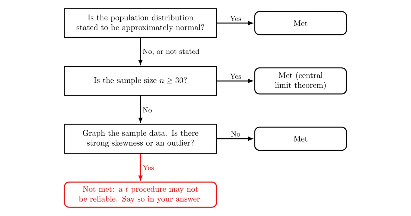
4.4 - Setting Up a Test for a Population Mean or Population Mean Difference

Name each condition and tie it to the problem. "Randomization: the 25 bottles were randomly selected from today's production" earns credit; "the data are random" doesn't. Don't swap the conditions either: the 10% condition isn't about randomness, and the sample data condition isn't about how the data were collected.

In a randomized experiment with volunteers, nobody is sampled without replacement from a population, so the 10% condition doesn't apply. Random assignment satisfies the randomization condition, but the results only generalize to people like the volunteers.

Example 1: Are bottles underfilled?

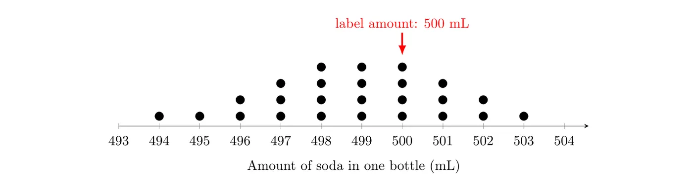
A bottling machine is supposed to fill soda bottles with 500 mL on average. A quality-control inspector worries that the machine is underfilling, so she randomly selects 25 of the 8,000 bottles filled today and measures the amount of soda in each. Set up a test for her question. Here is a dotplot of the 25 amounts:

State: she suspects underfilling, so the alternative is one-sided:

H_0: \mu = 500 \qquad H_a: \mu < 500

where

\mu

= the true mean amount of soda (mL) in all bottles filled by this machine today.

Plan: one quantitative variable (amount of soda), one sample, and

\sigma

unknown, so use a one-sample

t

-test for a population mean. Check the conditions:

Randomization: the 25 bottles were randomly selected from today's production.

10%: $25 \le 10\%(8{,}000) = 800$ .

Sample data: $n = 25 < 30$ , but the dotplot is roughly symmetric with no outliers, so this condition is met.

All three conditions are met, so a one-sample

t

-test is appropriate. Topic 4.5 finishes this test.

Example 2: Caffeine and reaction time (matched pairs)

A researcher recruits 14 adult volunteers. Each volunteer takes a reaction-time test twice, on different days: once an hour after a caffeine pill and once an hour after an identical-looking placebo pill. A coin flip decides which pill each person gets first. The reaction times (ms) are:

Volunteer	Placebo	Caffeine	Difference (caffeine minus placebo)
1	268	235	$-33$
2	295	271	$-24$
3	310	304	$-6$
4	252	234	$-18$
5	281	266	$-15$
6	274	282	8
7	302	290	$-12$
8	289	279	$-10$
9	263	259	$-4$
10	318	291	$-27$
11	277	275	$-2$
12	291	304	13
13	259	270	11
14	284	273	$-11$

The researcher wants to know whether caffeine changes mean reaction time. Set up a test.

State: the question asks whether caffeine changes reaction time and gives no direction, so the test is two-sided:

H_0: \mu_d = 0 \qquad H_a: \mu_d \ne 0

where

\mu_d

= the true mean difference in reaction time (caffeine minus placebo, in ms) for adults like these volunteers.

Plan: each volunteer gives two linked measurements, so this is a matched pairs design. Use a one-sample

t

-test for a population mean difference on the 14 differences. Check the conditions:

Randomization: the order of the two pills was randomly assigned for each volunteer. (The volunteers weren't a random sample, so the results apply to adults like them, not to all adults.)

10%: doesn't apply. This is an experiment, not a sample drawn without replacement from a population.

Sample data: there are only 14 differences, so graph them. The dotplot of the differences is roughly symmetric with no outliers.

A one-sample

t

-test on the differences is appropriate. Topic 4.5 finishes this test.

Example 3: Which test?

Name the procedure for each situation.

A random sample of 40 college students reports their hours of sleep per week. Is the mean less than 56 hours? Answer: a one-sample $t$ -test for a population mean.

Twenty runners each run a mile on a track and on a treadmill, in random order. Is there a mean difference in their times? Answer: a one-sample $t$ -test for a population mean difference (paired), since each runner gives two linked times.

Forty patients are randomly assigned, 20 each, to a new drug or a standard drug, and the drop in blood pressure is recorded. Does the new drug work better? Answer: a two-sample $t$ -test for $\mu_1 - \mu_2$ . The groups are separate people, so the data aren't paired (Topics 4.9 and 4.10).

In a random sample of 500 voters, is the proportion who support a ballot measure more than 50%? Answer: a one-sample $z$ -test for a population proportion (Unit 3). The variable is categorical, not quantitative.

Common mistakes

Writing hypotheses with statistics. $H_0: \bar{x} = 500$ is wrong; it must be $H_0: \mu = 500$ .

Analyzing paired data with a two-sample test, or the reverse.

Choosing the direction of $H_a$ after looking at the data.

Skipping the parameter definition, or defining $\mu_d$ without the order of subtraction.

Listing conditions without checking them in context, or using a $t$ procedure on a small sample that is strongly skewed or has outliers.

Switching to a $z$ -test because the sample is large. When $\sigma$ is unknown, it's a $t$ -test at any sample size.

Back Next