4.10 - Carrying Out a Test for the Difference Between Two Population Means

Overview

With the test set up (Topic 4.9), what's left is computing a test statistic, finding the

p

-value, and making a decision in context. The structure is the same as every significance test in this course: State, Plan, Do, Conclude. This topic covers the Do and Conclude steps for the two-sample

t

-test, including how to interpret the

p

-value.

The test statistic

The test statistic measures how far the observed difference in sample means is from the null value of 0, in standard errors:

t = \frac{(\bar{x}_1 - \bar{x}_2) - 0}{\sqrt{\dfrac{s_1^2}{n_1} + \dfrac{s_2^2}{n_2}}}

This is the formula sheet's standardized test statistic,

\frac{\text{statistic} - \text{parameter}}{\text{standard error of the statistic}}

, with the statistic

\bar{x}_1 - \bar{x}_2

and the null value 0. A value of

t = 2.55

means the sample difference is 2.55 standard errors above what

H_0

predicts.

When the null hypothesis is true,

t

has a

t

-distribution. Technology finds the degrees of freedom (the same df as the two-sample

t

-interval), and they fall between the smaller of

n_1 - 1

and

n_2 - 1

and

n_1 + n_2 - 2

. Without technology, use the smaller of

n_1 - 1

and

n_2 - 1

Finding the $p$ -value

The

p

-value is the area under the

t

-distribution beyond the test statistic, in the direction of

H_a

4.10 - Carrying Out a Test for the Difference Between Two Population Means

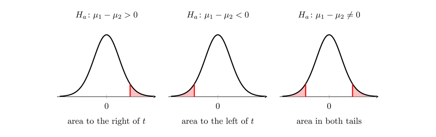
$H_a\colon \mu_1 - \mu_2 > 0$ : the area to the right of $t$ .

$H_a\colon \mu_1 - \mu_2 < 0$ : the area to the left of $t$ .

$H_a\colon \mu_1 - \mu_2 \neq 0$ : the area in both tails, beyond $-|t|$ and $|t|$ . That's double the one-tail area.

With technology

On a TI-84, press STAT, arrow to TESTS, and choose 4:2-SampTTest. Enter the data or the summary statistics, choose the alternative (

\neq

<

, or

>

), set Pooled: No, and select Calculate. The output shows

t

p

, and df. You can also find a tail area directly with tcdf(lower, upper, df), for example tcdf(2.55, 1E99, 21.2) for the right tail beyond 2.55.

With Table B

Use the conservative df (the smaller of

n_1 - 1

and

n_2 - 1

, moving to the next smaller row if that df isn't in the table). Find where

|t|

falls in that row; the column headings give bounds on the one-tail area. Double the bounds for a two-sided test. A table gives a range, like

0.01 < p < 0.02

, which is enough to compare with

\alpha

Interpreting the $p$ -value

The

p

-value is the probability of getting a test statistic as extreme as, or more extreme than, the one observed (in the direction of

H_a

), given that the null hypothesis is true. For two means, assuming

H_0

is true means assuming the two population means are equal. A good interpretation follows this pattern:

Assuming the true mean [variable] is the same for [population 1] and [population 2], there is a [ $p$ -value] probability of getting a difference in sample means of [observed difference] or more [in the direction of the alternative] by chance alone.

An interpretation that leaves out the "assuming

H_0

is true" part is incomplete. And the

p

-value is not the probability that

H_0

is true.

Making a decision and a conclusion

A formal decision explicitly compares the

p

-value to the significance level

\alpha

If the $p$ -value $\leq \alpha$ , reject $H_0$ . There is convincing evidence for $H_a$ .

If the $p$ -value $> \alpha$ , fail to reject $H_0$ . There is not convincing evidence for $H_a$ .

Then write the conclusion in context: in terms of

H_a

, with non-definitive language, naming the parameters and the populations. For example:

Because the $p$ -value of 0.0093 is less than $\alpha = 0.05$ , we reject $H_0$ . There is convincing statistical evidence that the true mean height after three weeks is greater for bean plants like these grown with the plant food than for bean plants like these grown with plain water.

The results of the test are the statistical reasoning behind the answer to the investigative question about the two populations, so state that answer in the problem's own words. A few more rules:

Never "accept $H_0$ " or say the test "proves" anything. Failing to reject means the evidence wasn't strong enough, not that the means are equal.

Talk about the population means ("the true mean," "all phone players"), not the sample means.

For a randomized experiment, rejecting $H_0$ supports a cause-and-effect conclusion for units like those in the study. For random samples from two populations, the conclusion applies to those populations but doesn't show cause and effect.

Example 1: Plant food for bean plants

This finishes the test set up in Topic 4.9, Example 2. Twenty-four bean seedlings were randomly assigned to plant food or plain water, 12 each. Heights after three weeks, in cm:

Group	Heights (cm)
Plant food	23.1, 25.4, 21.8, 26.0, 24.7, 22.9, 27.3, 24.2, 25.8, 23.6, 26.5, 24.9
Water only	22.6, 23.9, 21.3, 24.8, 23.0, 20.9, 25.1, 22.7, 23.8, 21.9, 24.4, 23.2

Is there convincing evidence at

\alpha = 0.05

that the plant food increases the mean height after three weeks?

State:

H_0\colon \mu_F - \mu_W = 0

and

H_a\colon \mu_F - \mu_W > 0

, where

\mu_F

and

\mu_W

are the true mean heights after three weeks for bean plants like these grown with plant food and with plain water. We'll use

\alpha = 0.05

Plan: Two-sample

t

-test for

\mu_F - \mu_W

. Conditions:

Randomization: the treatments were randomly assigned to the 24 seedlings.

10%: not needed, because this is a randomized experiment.

Sample data: both groups have 12 plants, and boxplots of both groups (Topic 4.9) show no outliers and no strong skewness.

Do: From the data,

\bar{x}_F \approx 24.683

s_F \approx 1.6264

\bar{x}_W \approx 23.133

, and

s_W \approx 1.3364

cm.

t = \frac{24.683 - 23.133}{\sqrt{\dfrac{1.6264^2}{12} + \dfrac{1.3364^2}{12}}} = \frac{1.550}{0.6077} \approx 2.55

Technology gives df

\approx 21.20

and a

p

-value of

P(t \geq 2.55) \approx 0.0093

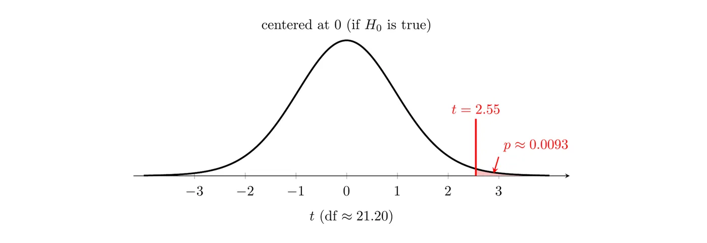
Without technology: df

= 12 - 1 = 11

. In the df = 11 row of Table B, 2.55 falls between 2.328 (tail area 0.02) and 2.718 (tail area 0.01), so

0.01 < p < 0.02

Interpret the

p

-value: Assuming the plant food has no effect on mean height (the true means are equal), there is about a 0.0093 probability of getting a difference in sample means of 1.55 cm or more in favor of the plant food just from the random assignment.

Conclude: Because

p \approx 0.0093 \leq \alpha = 0.05

, we reject

H_0

. There is convincing statistical evidence that the true mean height after three weeks is greater for bean plants like these grown with the plant food than for those grown with plain water. Because the treatments were randomly assigned, this is evidence that the plant food causes taller growth, on average, for plants like these.

Example 2: Phone and console players (AP-style)

This finishes the test set up in Topic 4.9, Example 1. The samples gave these results:

Group	$n$	$\bar{x}$ (minutes)	$s$ (minutes)
Phone players	50	38.5	14.2
Console players	42	43.1	17.9

Is there convincing evidence at

\alpha = 0.05

that the mean session length differs between phone and console players?

State:

H_0\colon \mu_P - \mu_C = 0

and

H_a\colon \mu_P - \mu_C \neq 0

, where

\mu_P

and

\mu_C

are the true mean session lengths, in minutes, for all phone players and all console players of the game. We'll use

\alpha = 0.05

Plan: Two-sample

t

-test for

\mu_P - \mu_C

. Conditions (checked in Topic 4.9): two independent random samples; each sample is far less than 10% of its population; and both samples have at least 30 players, so the skewed session lengths aren't a problem.

Do:

t = \frac{38.5 - 43.1}{\sqrt{\dfrac{14.2^2}{50} + \dfrac{17.9^2}{42}}} = \frac{-4.6}{\sqrt{4.033 + 7.629}} = \frac{-4.6}{3.415} \approx -1.35

Technology gives df

\approx 77.6

and a two-sided

p

-value of about 0.182 (0.091 in each tail).

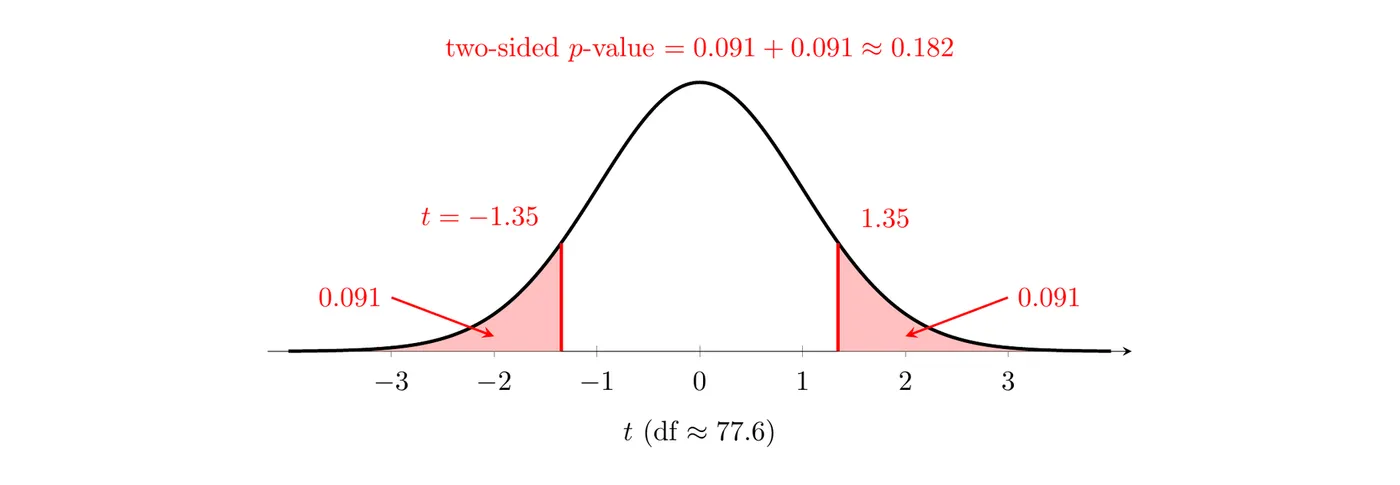
Without technology: df

= 42 - 1 = 41

, which isn't in Table B, so use the df = 40 row.

|t| = 1.35

falls between 1.303 (tail area 0.10) and 1.684 (tail area 0.05), so one tail is between 0.05 and 0.10, and the two-sided

p

-value is between 0.10 and 0.20.

Interpret the

p

-value: Assuming the true mean session length is the same for phone and console players, there is about a 0.182 probability of getting a difference in sample means of 4.6 minutes or more, in either direction, by chance alone.

Conclude: Because

p \approx 0.182 > \alpha = 0.05

, we fail to reject

H_0

. There is not convincing statistical evidence that the true mean session length differs between all phone players and all console players of this game.

Notice what this does not say: it doesn't say the means are equal. The console players in the sample averaged 4.6 minutes more, but a difference that size isn't unusual by chance when the true means are equal. A 95% two-sample

t

-interval for

\mu_P - \mu_C

(-11.40, 2.20)

minutes, which contains 0, matching the decision.

Common mistakes

Skipping the explicit comparison. Write " $p = 0.0093 \leq 0.05$ ," not just "the $p$ -value is small."

Concluding about the samples ("the plant food group had a larger mean") instead of the populations, or using definite words like "proves."

Accepting the null hypothesis. After a large $p$ -value, you fail to reject $H_0$ ; you never accept it.

Getting the tail wrong. Use the direction of $H_a$ , and double the one-tail area for a two-sided test.

Leaving the assumption out of a $p$ -value interpretation. It must say the $p$ -value is computed assuming $H_0$ is true. It is not the probability that $H_0$ is true.

Using z instead of t, or turning pooling on in the calculator.

A sign that doesn't match the setup. If $H_a$ is about $\mu_F - \mu_W$ , compute $\bar{x}_F - \bar{x}_W$ in that order.

Back Next