4.1 - Sampling Distributions for Sample Means

Overview

In Unit 3 you saw that a sample proportion

\hat{p}

changes from sample to sample in a predictable way. Sample means behave the same way. If you take every possible random sample of the same size from a population and compute

\bar{x}

for each one, those values of

\bar{x}

form the sampling distribution of the sample mean. This topic gives its center, spread, and shape, and shows how to use it to find probabilities. Every confidence interval and test in Unit 4 is built on it.

Three distributions to keep straight

A sampling distribution is the distribution of a statistic's values over all possible samples of a given size from a population (Topic 2.12). For a quantitative variable, the statistic is usually the sample mean

\bar{x}

. Every problem about

\bar{x}

involves three distributions, so keep them straight:

Distribution	What it shows	Center and spread
Population	The variable's value for every individual	$\mu$ and $\sigma$ (parameters)
One sample	The $n$ values you actually collected	$\bar{x}$ and $s$ (statistics)
Sampling distribution of $\bar{x}$	The values of $\bar{x}$ from all possible samples of size $n$	$\mu_{\bar{x}}$ and $\sigma_{\bar{x}}$

Center and spread

For a population with mean

\mu

and standard deviation

\sigma

, when the sampled values are independent, the sampling distribution of

\bar{x}

has

\mu_{\bar{x}} = \mu \qquad \text{and} \qquad \sigma_{\bar{x}} = \frac{\sigma}{\sqrt{n}}

Center: $\mu_{\bar{x}} = \mu$ . The sample mean is an unbiased estimator of $\mu$ . Some samples land above $\mu$ and some below, but they don't systematically overshoot or undershoot.

Spread: $\sigma_{\bar{x}} = \sigma/\sqrt{n}$ . Averaging cancels out some variability, because an unusually high value in a sample tends to be offset by lower ones. So means vary less than individual values, and bigger samples vary less still.

Because

n

sits under a square root, you have to quadruple the sample size to cut

\sigma_{\bar{x}}

in half. Going from

n = 25

n = 100

halves it. Both formulas are on the AP formula sheet.

Conditions

The formula

\sigma_{\bar{x}} = \sigma/\sqrt{n}

assumes the observations are independent. When you sample without replacement (the usual case), two conditions make that safe:

Randomization condition: the data should be collected using a random sample. This makes the sample representative and the values independent of each other.

10% condition: when sampling without replacement, the population size must be at least 10 times the sample size, $n \le 10\%N$ , where $N$ is the population size and $n$ is the sample size. Removing a few individuals from a big population barely changes who's left, so the observations are close enough to independent and the formula for $\sigma_{\bar{x}}$ is accurate.

Keep the two apart. The randomization condition is about how the data were collected. The 10% condition is about how much of the population you sampled. Mixing them up (for example, calling the 10% condition a randomness check) is one of the most common errors on the AP exam.

Shape

When the population is normal

If the population distribution of the variable can be modeled by a normal distribution, the sampling distribution of

\bar{x}

is also normal, regardless of the sample size. Even means of samples of 2 are normally distributed.

When the population isn't normal: the central limit theorem

If the population is not normal, or you don't know its shape, the central limit theorem (CLT) says the sampling distribution of

\bar{x}

is approximately normal as long as the sample is large enough. The AP rule of thumb is

n \ge 30

. If the population is extremely skewed, a sample size much larger than 30 may be needed before the sampling distribution looks normal.

The figure shows this for a population of drive-thru service times that is skewed right, with

\mu = 3.8

minutes and

\sigma = 2.5

minutes. In every panel the center stays at 3.8. The spread shrinks by a factor of

\sqrt{n}

. The shape goes from clearly skewed (the population) to slightly skewed (

n = 5

) to very close to normal (

n = 40

4.1 - Sampling Distributions for Sample Means

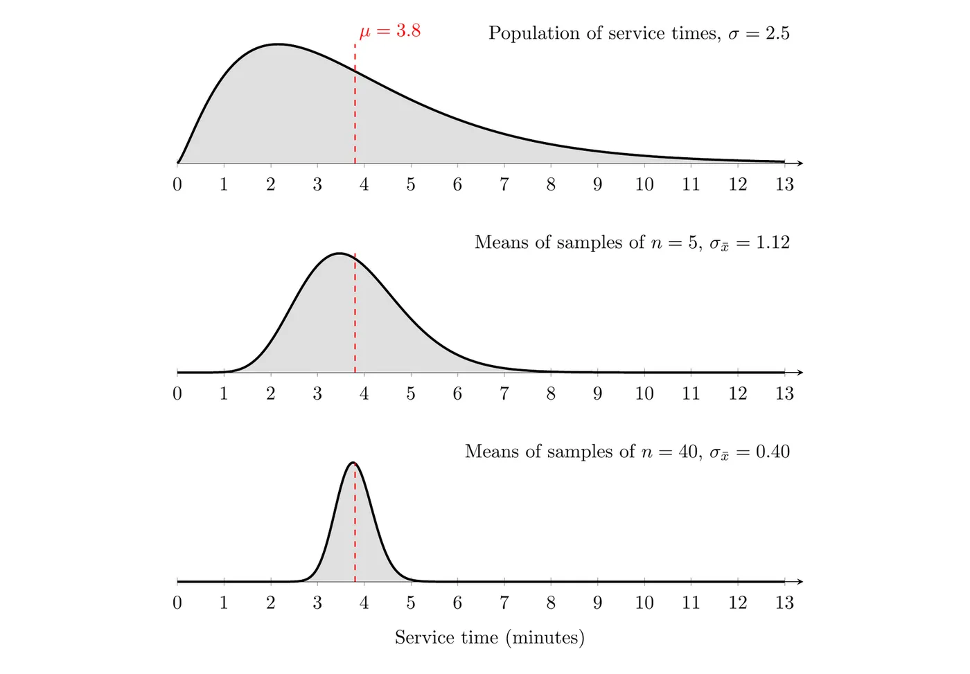
The CLT is about the sampling distribution of

\bar{x}

, not the population and not the sample. A large sample from a skewed population is still skewed. It's the distribution of the sample means that becomes approximately normal.

Population shape	Sample size	Shape of the sampling distribution of $\bar{x}$
Normal	Any $n$	Normal
Not normal, or unknown	$n \ge 30$	Approximately normal (CLT)
Not normal, or unknown	$n < 30$	Can't assume normal; it depends on the population's shape

Finding and interpreting probabilities

When the sampling distribution of

\bar{x}

is normal or approximately normal, standardize with the sampling distribution's mean and standard deviation, not the population's:

z = \frac{\bar{x} - \mu_{\bar{x}}}{\sigma_{\bar{x}}} = \frac{\bar{x} - \mu}{\sigma / \sqrt{n}}

Then use Table A or technology. On a TI-84, normalcdf(lower, upper, mean, SD) with mean

\mu

and SD

\sigma/\sqrt{n}

gives the area directly.

Interpret every mean, standard deviation, and probability in the context of the specific population. For example,

\sigma_{\bar{x}} = 0.4

hours in Example 1 below means: across all possible random samples of 9 phones, the sample mean battery life typically varies from the population mean of 12.5 hours by about 0.4 hours.

Example 1: One phone vs. a sample of nine

The battery life of a certain phone model is approximately normal with mean

\mu = 12.5

hours and standard deviation

\sigma = 1.2

hours. A reviewer takes a random sample of 9 phones from a large shipment. (a) Find the mean and standard deviation of the sampling distribution of

\bar{x}

. (b) Find the probability that one randomly chosen phone's battery lasts less than 12 hours. (c) Find the probability that the mean battery life of the 9 phones is less than 12 hours.

(a) The sample is random, and 9 phones is far less than 10% of a large shipment, so the observations are close enough to independent.

\mu_{\bar{x}} = \mu = 12.5 \text{ hours} \qquad \sigma_{\bar{x}} = \frac{1.2}{\sqrt{9}} = \frac{1.2}{3} = 0.4 \text{ hours}

The population is normal, so the sampling distribution of

\bar{x}

is normal even though

n = 9

is small.

(b) One phone comes from the population distribution, so use

\sigma = 1.2

z = \frac{12 - 12.5}{1.2} \approx -0.42 \qquad P(X < 12) \approx 0.3385

(Technology gives 0.3385. Table A with

z = -0.42

gives 0.3372. Either is fine.)

(c) The mean of 9 phones comes from the sampling distribution, so use

\sigma_{\bar{x}} = 0.4

z = \frac{12 - 12.5}{0.4} = -1.25 \qquad P(\bar{x} < 12) \approx 0.1056

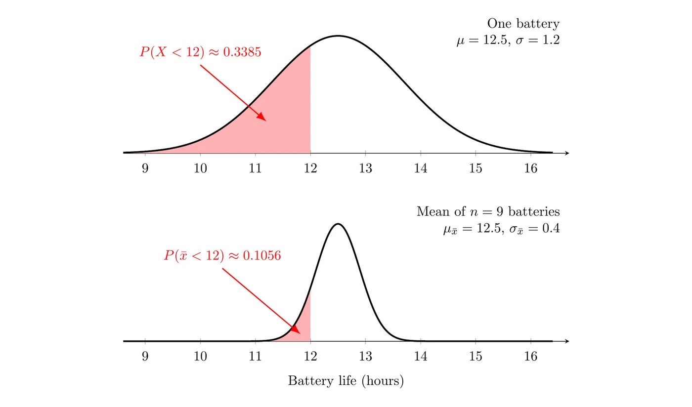
Answer: About 34% of individual phones have a battery life under 12 hours, but only about 11% of random samples of 9 phones have a mean battery life under 12 hours. Means of several phones cluster more tightly around 12.5 hours than single phones do, so a mean this low is less likely.

Example 2: A skewed population (AP-style)

At a fast-food drive-thru, service times are skewed to the right, with mean

\mu = 3.8

minutes and standard deviation

\sigma = 2.5

minutes. The manager takes a random sample of 40 of the 2,000 orders from this month. (a) Is the sampling distribution of

\bar{x}

approximately normal? Explain. (b) Find the probability that the sample mean service time is more than 4.5 minutes. (c) Could you use a normal model to find the probability that one randomly chosen order takes more than 4.5 minutes? Explain.

(a) Yes. The population is skewed, but

n = 40 \ge 30

, so by the central limit theorem the sampling distribution of

\bar{x}

is approximately normal. The other conditions hold too: the sample is random, and

40 \le 10\%(2{,}000) = 200

(b) Find the mean and standard deviation of

\bar{x}

, then standardize:

\mu_{\bar{x}} = 3.8 \qquad \sigma_{\bar{x}} = \frac{2.5}{\sqrt{40}} \approx 0.395

z = \frac{4.5 - 3.8}{0.395} \approx 1.77 \qquad P(\bar{x} > 4.5) \approx 0.038

Answer: About 3.8% of all random samples of 40 orders would have a mean service time above 4.5 minutes. So if the manager's sample mean came out above 4.5 minutes, that would be unusual if the true mean were still 3.8 minutes, and it would suggest service has slowed down.

(c) No. A single service time comes from the population distribution, which is skewed right, not normal. The CLT only makes the distribution of the sample mean approximately normal.

Example 3: Choosing a sample size

For the drive-thru in Example 2, how large a sample would make

\sigma_{\bar{x}}

at most 0.25 minutes?

\frac{2.5}{\sqrt{n}} \le 0.25 \;\Rightarrow\; \sqrt{n} \ge 10 \;\Rightarrow\; n \ge 100

Answer: The manager needs a random sample of at least 100 orders. That still meets the 10% condition, since

100 \le 200

Common mistakes

Using $\sigma$ instead of $\sigma/\sqrt{n}$ when the question is about a sample mean. Ask yourself: is this about one individual, or the mean of a sample?

Saying the CLT makes the population or the sample normal. It only applies to the sampling distribution of $\bar{x}$ .

Using a normal model for $\bar{x}$ when $n < 30$ and the population isn't known to be normal.

Mixing up the randomization condition and the 10% condition, or skipping the 10% condition when sampling without replacement.

Thinking a bigger sample moves the center. A larger $n$ shrinks the spread, but $\mu_{\bar{x}} = \mu$ for every sample size.

Giving a probability with no context. Say what it means for the specific population (phones, orders, students).

Back Next