4.6 - Sampling Distributions for the Difference Between Two Sample Means

Overview

Many statistical questions compare two groups. Do students at one school spend more time on screens than students at another? Are apples from one orchard heavier than apples from another? To answer them, you take a random sample from each population and compare the sample means using the difference

\bar{x}_1 - \bar{x}_2

. This topic describes how that difference behaves from sample to sample: its center, its spread, and when its distribution is normal. Everything in Topics 4.7 to 4.10 is built on it.

Two samples, one statistic

Picture two populations. Population 1 has mean

\mu_1

and standard deviation

\sigma_1

. Population 2 has mean

\mu_2

and standard deviation

\sigma_2

. Take a random sample of size

n_1

from population 1, take a separate random sample of size

n_2

from population 2, and compute the difference in sample means:

\bar{x}_1 - \bar{x}_2

This difference is a statistic, so it changes from one pair of samples to the next. The sampling distribution of

\bar{x}_1 - \bar{x}_2

is the distribution of its values over all possible pairs of samples of sizes

n_1

and

n_2

. It works the same way as the sampling distribution of

\hat{p}_1 - \hat{p}_2

in Topic 3.9, with means in place of proportions.

Mean and standard deviation of the sampling distribution

For two independent populations, when the sampled values are independent, the sampling distribution of

\bar{x}_1 - \bar{x}_2

has this mean and standard deviation:

\mu_{\bar{x}_1 - \bar{x}_2} = \mu_1 - \mu_2

\sigma_{\bar{x}_1 - \bar{x}_2} = \sqrt{\frac{\sigma_1^2}{n_1} + \frac{\sigma_2^2}{n_2}}

Both formulas are on the AP formula sheet, in the table "Sampling Distributions for Means." On the exam you use them to describe the sampling distribution and to find probabilities about

\bar{x}_1 - \bar{x}_2

The center: no bias

The mean of the sampling distribution is exactly the true difference

\mu_1 - \mu_2

. Some pairs of samples overestimate the difference and some underestimate it, but on average they hit it. That makes

\bar{x}_1 - \bar{x}_2

an unbiased estimator of

\mu_1 - \mu_2

The spread: variances add

Each sample mean has its own sampling variability. From Topic 4.1,

\sigma_{\bar{x}} = \frac{\sigma}{\sqrt{n}}

, so the variance (the square of the standard deviation) of each sample mean is

\frac{\sigma_1^2}{n_1}

\frac{\sigma_2^2}{n_2}

. When you subtract two independent sample means, their random errors don't cancel out. Either mean can land high or low, and both errors end up in the difference. So the variances add, and the standard deviation is the square root of the sum:

\sigma_{\bar{x}_1 - \bar{x}_2} = \sqrt{\sigma_{\bar{x}_1}^2 + \sigma_{\bar{x}_2}^2} = \sqrt{\frac{\sigma_1^2}{n_1} + \frac{\sigma_2^2}{n_2}}

Add variances, never standard deviations. Writing $\sigma_{\bar{x}_1} + \sigma_{\bar{x}_2}$ is wrong. Square each one, add, then take the square root.

It's a plus sign even though the statistic is a difference. Subtracting two random quantities makes the result more variable, not less.

Bigger samples, less spread. Increasing $n_1$ or $n_2$ shrinks its term, so $\bar{x}_1 - \bar{x}_2$ varies less.

Conditions for using the formulas

The standard deviation formula assumes the two samples are independent of each other and that the values inside each sample are independent. When you sample without replacement, two conditions make that reasonable:

Randomization condition: the data should be collected using two independent random samples, one from each population. Independent means that who gets picked for one sample has nothing to do with who gets picked for the other. Measuring the same students twice is not independent; that's paired data, analyzed as one sample of differences (Topic 4.2).

10% condition: each sample size must be at most 10% of its population size: $n_1 \leq 10\%N_1$ and $n_2 \leq 10\%N_2$ , where $N_1$ and $N_2$ are the population sizes. Sampling without replacement makes the values in a sample slightly dependent. When the sample is a small slice of the population, that dependence is small enough to ignore.

Experiments work differently. If the data come from an experiment, only the randomization condition is needed, and it means the treatments were randomly assigned to the experimental units. No population is being sampled, so there's no 10% condition. Random assignment is what makes the two groups independent, and it's the source of the chance variation that the formulas describe.

On the exam, name each condition and tie it to the problem with numbers, for example "40 is less than 10% of the 1,850 students at North." Keep the randomization and 10% conditions separate; mixing them up is a common error.

When the sampling distribution is normal

The shape of the sampling distribution of

\bar{x}_1 - \bar{x}_2

depends on the populations and the sample sizes:

Populations	Sample sizes	Sampling distribution of $\bar{x}_1 - \bar{x}_2$
Both can be modeled by a normal distribution	Any sizes	Normal
At least one can't be modeled by a normal distribution (or the shape is unknown)	$n_1 \geq 30$ and $n_2 \geq 30$	Approximately normal
A population that isn't normal (or whose shape is unknown)	That population's sample has fewer than 30 values	Don't assume it's normal

Here's why. Each

\bar{x}

is normal when its population is normal, or approximately normal by the central limit theorem when its sample is large (Topic 4.1), and the difference of two independent normal variables is normal too. An extremely skewed population may need a sample much larger than 30. A large sample changes the shape of the sampling distribution, not the shape of the population.

Interpreting in context

The mean, standard deviation, and probabilities from this sampling distribution should always be interpreted for the specific populations in the problem. Use these sentence frames, filled in with the real context:

Quantity	What it means
Mean, $\mu_{\bar{x}_1 - \bar{x}_2}$	Across all possible pairs of random samples of these sizes, the difference in sample mean [variable] ([group 1] minus [group 2]) averages $\mu_1 - \mu_2$ .
Standard deviation, $\sigma_{\bar{x}_1 - \bar{x}_2}$	The difference in sample mean [variable] typically varies by about $\sigma_{\bar{x}_1 - \bar{x}_2}$ [units] from $\mu_1 - \mu_2$ in repeated random sampling.
A probability	The proportion of all possible pairs of random samples that give a difference in sample means in the stated range.

Example 1: Apple weights from two orchards

Apple weights at Orchard A are approximately normal with mean 150 g and standard deviation 20 g. At Orchard B they are approximately normal with mean 140 g and standard deviation 25 g. A grocer picks a random sample of 10 apples from Orchard A and an independent random sample of 12 apples from Orchard B. Find the mean and standard deviation of the sampling distribution of

\bar{x}_A - \bar{x}_B

, then find the probability that the Orchard B sample has the larger mean weight.

Step 1: find the mean.

\mu_{\bar{x}_A - \bar{x}_B} = \mu_A - \mu_B = 150 - 140 = 10 \text{ g}

Step 2: find the standard deviation.

\sigma_{\bar{x}_A - \bar{x}_B} = \sqrt{\frac{20^2}{10} + \frac{25^2}{12}} = \sqrt{40 + 52.083} = \sqrt{92.083} \approx 9.60 \text{ g}

Step 3: check the conditions and the shape. The two samples are random and independent, and each orchard has far more than 100 and 120 apples, so the 10% condition holds. Both populations are approximately normal, so the sampling distribution of

\bar{x}_A - \bar{x}_B

is approximately normal even though both samples are small.

Step 4: find the probability. "Orchard B has the larger sample mean" means

\bar{x}_A - \bar{x}_B < 0

z = \frac{0 - 10}{9.60} \approx -1.04

P(\bar{x}_A - \bar{x}_B < 0) = P(z < -1.04) \approx 0.149

On a TI-84, normalcdf(-1E99, 0, 10, 9.596) gives the same answer, about 0.149.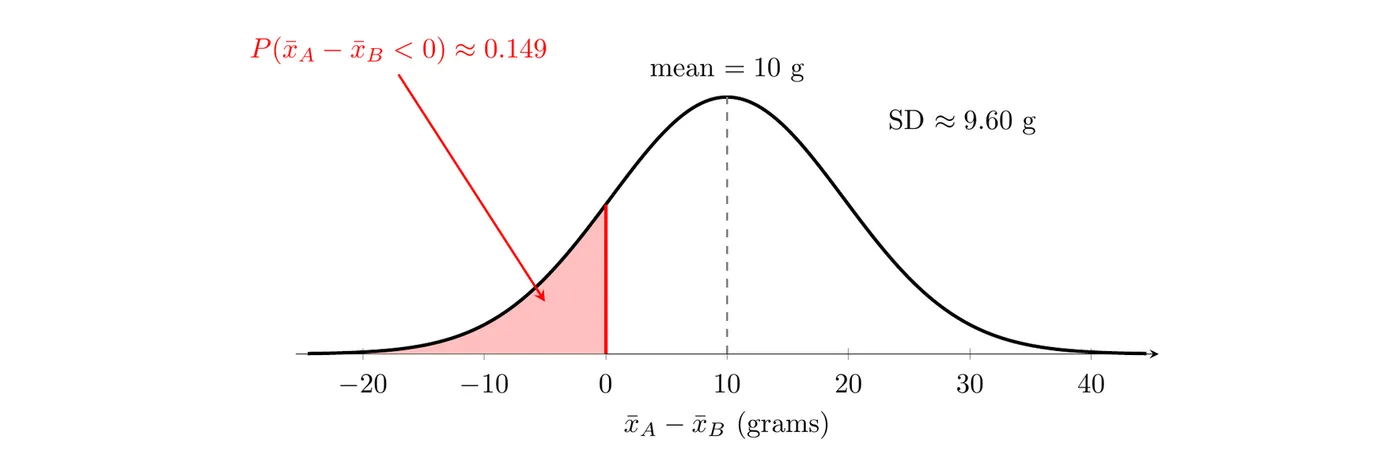

4.6 - Sampling Distributions for the Difference Between Two Sample Means

Answer: The difference in sample mean weights (A minus B) has mean 10 g and standard deviation about 9.60 g. In about 14.9% of all possible pairs of random samples like these, the 12 apples from Orchard B would have a higher mean weight than the 10 apples from Orchard A, even though Orchard A's apples are heavier on average. Small samples can easily point the wrong way.

Example 2: Screen time at two high schools (AP-style)

At North High (1,850 students), daily screen time has mean 215 minutes and standard deviation 70 minutes. At South High (1,420 students), the mean is 190 minutes and the standard deviation is 80 minutes. Both distributions are strongly skewed to the right. A researcher selects a random sample of 40 North students and an independent random sample of 35 South students.

Describe the sampling distribution of $\bar{x}_N - \bar{x}_S$ (shape, center, and variability), and justify the shape.

Assuming these population values are correct, find the probability that North's sample mean is at least 60 minutes higher than South's. Would a difference that large be surprising?

Part 1, conditions. The data come from two independent random samples, so the randomization condition is met. Also

40 \leq 10\%(1{,}850) = 185

and

35 \leq 10\%(1{,}420) = 142

, so the 10% condition is met.

Center:

\mu_{\bar{x}_N - \bar{x}_S} = 215 - 190 = 25 \text{ minutes}

Variability:

\sigma_{\bar{x}_N - \bar{x}_S} = \sqrt{\frac{70^2}{40} + \frac{80^2}{35}} = \sqrt{122.5 + 182.857} = \sqrt{305.357} \approx 17.47 \text{ minutes}

Shape: the populations are strongly skewed, so they can't be modeled by normal distributions. But

n_N = 40 \geq 30

and

n_S = 35 \geq 30

, so the sampling distribution of

\bar{x}_N - \bar{x}_S

is approximately normal.

In context: across all possible pairs of random samples of 40 North students and 35 South students, the difference in sample mean daily screen time (North minus South) averages 25 minutes and typically varies from 25 minutes by about 17.47 minutes.

Part 2. Standardize 60 and find the area to the right.

z = \frac{60 - 25}{17.47} \approx 2.00

P(\bar{x}_N - \bar{x}_S \geq 60) = P(z \geq 2.00) \approx 0.023

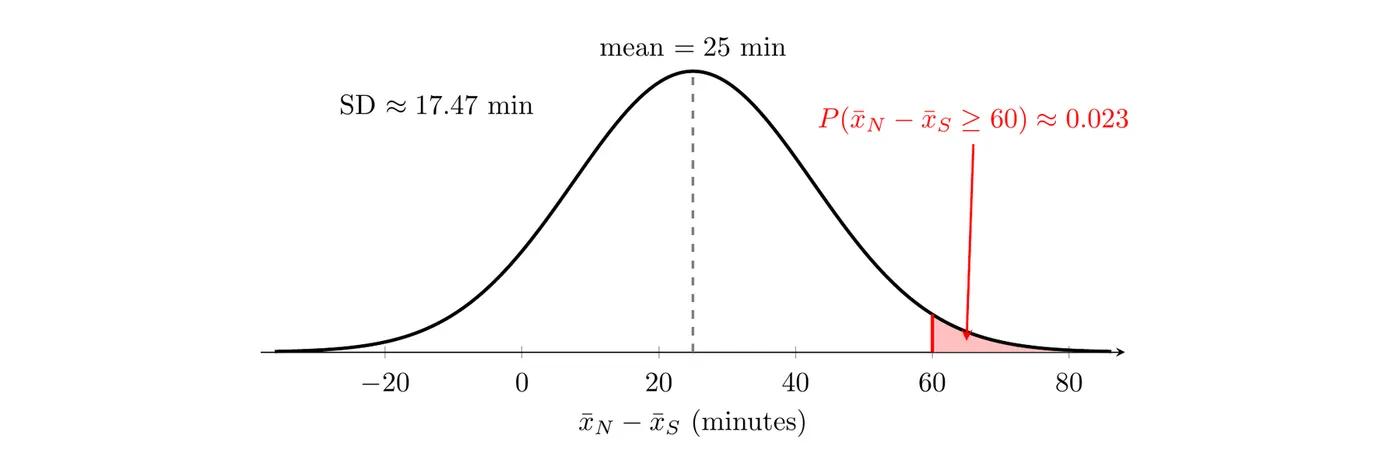
Answer: If the population means really are 215 and 190 minutes, only about 2.3% of all possible pairs of random samples like these would show North's sample mean at least 60 minutes higher than South's. That's unusual, so seeing a 60-minute gap would make us doubt the stated population values (the true difference may be larger than 25 minutes). A significance test makes this kind of reasoning formal in Topic 4.10.

SE_{\bar{x}_1 - \bar{x}_2} = \sqrt{\frac{s_1^2}{n_1} + \frac{s_2^2}{n_2}}

Estimating

\sigma

with

s

adds extra uncertainty, so inference for two means uses

t

-distributions instead of the standard normal. That leads to the two-sample

t

-interval (Topic 4.7) and the two-sample

t

-test (Topics 4.9 and 4.10).

Common mistakes

Adding standard deviations instead of variances: $\sqrt{a} + \sqrt{b}$ is not $\sqrt{a + b}$ .

Subtracting the variances because the statistic is a difference. The variances always add.

Mixing up the sample sizes. Each variance is divided by its own sample size: $\sigma_1^2$ by $n_1$ and $\sigma_2^2$ by $n_2$ .

Claiming normality without a reason. If a population isn't normal, you need its sample size to be at least 30. Saying "the population is normal because $n \geq 30$ " is also wrong: the sample size affects the sampling distribution, not the population.

Using this for paired data. Before-and-after measurements on the same people are not independent samples. Analyze the differences as one sample (Topic 4.2).

Switching the order of subtraction. If you define the difference as A minus B, keep A minus B in the mean, in the event you're finding the probability of, and in your interpretation.

Back Next