2.9 - Resistive Forces

Introduction to Resistive Forces

Resistive forces (also called drag or air resistance) are velocity-dependent forces that point opposite to an object’s velocity.

This one is calculus-heavy and usually doesn’t come up in algebra-based physics. Resistive force problems lean hard on differential equations and integration.

Mathematical Forms of Resistive Forces

Resistive forces usually get modeled one of two ways.

Linear Drag (proportional to velocity)

\vec{F}_r = -bv

\vec{F}_r = -kv

where: -

\vec{F}_r

= resistive force (N). -

b

k

= drag coefficient (kg/s). -

v

= speed of the object (m/s).

The negative sign says the force opposes the motion.

Quadratic Drag (proportional to velocity squared)

\vec{F}_r = -cv^2

where

c

is a different drag coefficient with units of kg/m.

Note: for most AP Physics C problems, you’ll use linear drag (

-bv

-kv

). The AP exam usually just hands you the drag coefficient as a constant instead of making you calculate it from physical properties.

Common Problem Structure on the AP Exam

Resistive force free-response questions usually follow this pattern:

Part A: draw a free body diagram.

Part B: write (but don’t solve) a differential equation for the motion.

Part C: find the terminal velocity.

Part D: solve the differential equation for velocity as a function of time.

Setting Up the Differential Equation

Start with Newton’s Second Law:

\sum F = ma

Since acceleration is the derivative of velocity:

a = \frac{dv}{dt}

the equation turns into:

\sum F = m\frac{dv}{dt}

That’s your differential equation, because it has the derivative

\frac{dv}{dt}

in it.

Example: Object Falling with Air Resistance

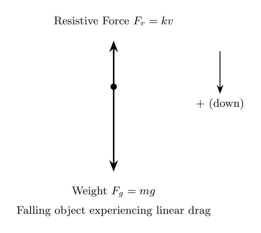
Taking downward as positive:

mg - kv = m\frac{dv}{dt}

That’s the differential equation for Part B.

Terminal Velocity

Terminal velocity is when the net force hits zero, so the acceleration is zero.

\sum F = 0

At terminal velocity, the forces balance:

F_g = F_r

For a falling object with linear drag:

mg = kv_t

Solve for terminal velocity:

v_t = \frac{mg}{k}

What’s happening: as the object falls and speeds up, the drag grows until it matches gravity. At that point the object stops accelerating and falls at a steady speed.

AP Physics C defines terminal velocity as the maximum speed an object reaches when a constant force (like gravity) and a resistive force act on it in opposite directions. That fits an object that starts slower than

v_t

. If something starts out faster than

v_t

(say it’s thrown straight down very hard), the drag is bigger than gravity at first, so it slows down toward

v_t

instead. Either way, it heads for the speed where the net force is zero.

Solving the Differential Equation

To get velocity as a function of time, you solve the differential equation with separation of variables and integration.

The General Process

Step 1: Start with the differential equation

mg - kv = m\frac{dv}{dt}

Step 2: Separate the variables (v’s on one side, t’s on the other)

Divide by

m

g - \frac{k}{m}v = \frac{dv}{dt}

Multiply both sides by

dt

and divide by

(g - \frac{kv}{m})

\frac{dv}{g - \frac{kv}{m}} = dt

Step 3: Integrate both sides

\int_0^{v(t)} \frac{dv}{g - \frac{kv}{m}} = \int_0^t dt

Step 4: Evaluate the integrals

The left side needs a substitution, or you can recognize it as a standard form:

\int \frac{dx}{a - bx} = -\frac{1}{b}\ln|a - bx| + C

Step 5: Solve for v(t)

This is where you lean on logarithm properties and exponential functions.

Example Problem: Object Dropped with Linear Drag

Problem: an object of mass

m

is dropped from rest near Earth’s surface. It feels a resistive force

F_r = kv

, where

v

is the speed and

k

is a constant. Take the direction of gravity as positive (downward).

Draw a free body diagram.

Write, but don’t solve, a differential equation for the velocity.

Derive an expression for the terminal velocity.

Derive an expression for the velocity as a function of time.

Part (a): Free Body Diagram

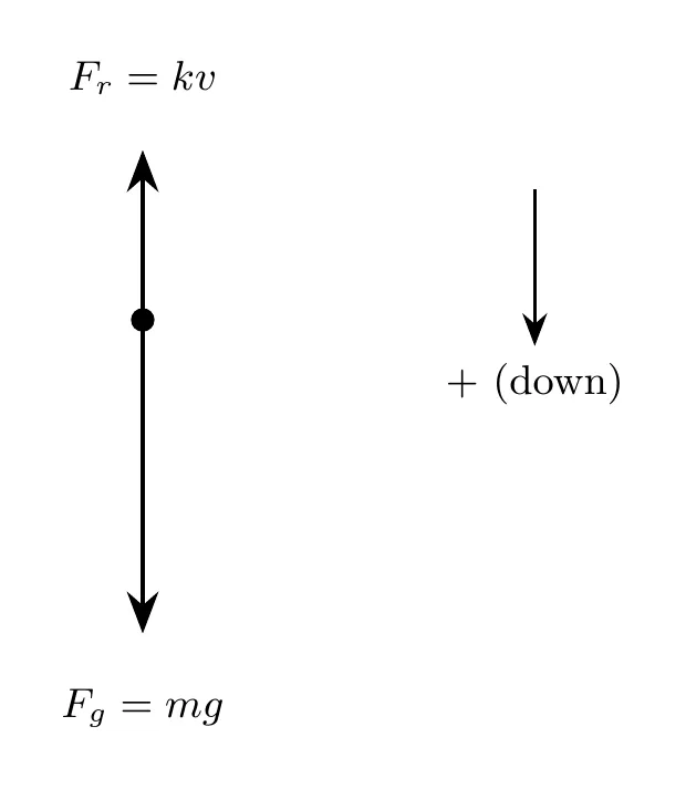
Part (b): Differential Equation

Apply Newton’s Second Law with downward as positive:

\sum F = ma

mg - kv = m\frac{dv}{dt}

Answer: the differential equation is:

mg - kv = m\frac{dv}{dt}

or, rearranged:

\frac{dv}{dt} = g - \frac{k}{m}v

Part (c): Terminal Velocity

At terminal velocity the acceleration is zero:

mg - kv_t = 0

mg = kv_t

v_t = \frac{mg}{k}

Answer: terminal velocity is

v_t = \frac{mg}{k}

Part (d): Velocity as a Function of Time

Step 1: Start with the differential equation

g - \frac{k}{m}v = \frac{dv}{dt}

Step 2: Separate the variables

\frac{dv}{g - \frac{kv}{m}} = dt

Step 3: Integrate both sides

\int_0^{v(t)} \frac{dv}{g - \frac{kv}{m}} = \int_0^t dt

Left side: use the formula

\int \frac{dx}{a - bx} = -\frac{1}{b}\ln|a - bx|

Here

a = g

and

b = \frac{k}{m}

\left[-\frac{m}{k}\ln\left|g - \frac{kv}{m}\right|\right]_0^{v(t)} = t

Step 4: Evaluate the definite integral

-\frac{m}{k}\ln\left(g - \frac{kv}{m}\right) - \left(-\frac{m}{k}\ln(g)\right) = t

-\frac{m}{k}\left[\ln\left(g - \frac{kv}{m}\right) - \ln(g)\right] = t

Step 5: Use logarithm properties

\ln(a) - \ln(b) = \ln\left(\frac{a}{b}\right)

-\frac{m}{k}\ln\left(\frac{g - \frac{kv}{m}}{g}\right) = t

-\frac{m}{k}\ln\left(1 - \frac{kv}{mg}\right) = t

Step 6: Solve for v

Multiply both sides by

-\frac{k}{m}

\ln\left(1 - \frac{kv}{mg}\right) = -\frac{kt}{m}

Exponentiate both sides:

1 - \frac{kv}{mg} = e^{-\frac{kt}{m}}

\frac{kv}{mg} = 1 - e^{-\frac{kt}{m}}

v = \frac{mg}{k}\left(1 - e^{-\frac{kt}{m}}\right)

Answer: the velocity as a function of time is:

v(t) = \frac{mg}{k}\left(1 - e^{-\frac{kt}{m}}\right)

Another way to write it, using terminal velocity:

Since

v_t = \frac{mg}{k}

v(t) = v_t\left(1 - e^{-\frac{kt}{m}}\right)

Heads up for the AP exam: pay attention to the form they want. If they ask for the answer “in terms of

m

g

k

, and fundamental constants,” use the first form. If they want it in terms of terminal velocity, use the second.

Physical Interpretation of the Solution

v(t) = \frac{mg}{k}\left(1 - e^{-\frac{kt}{m}}\right)

At t = 0:

v(0) = \frac{mg}{k}(1 - 1) = 0

The object starts from rest. ✓

As t → ∞:

e^{-\frac{kt}{m}} \to 0

v(\infty) = \frac{mg}{k}(1 - 0) = \frac{mg}{k} = v_t

The velocity eases up to terminal velocity. ✓

That exponential term

e^{-\frac{kt}{m}}

controls how fast the object closes in on terminal velocity: - Bigger

k

(more drag) means it gets there faster. - Bigger

m

(more inertia) means it gets there slower.

The combination

\frac{m}{k}

has units of seconds and is called the time constant,

\tau = \frac{m}{k}

. After one time constant,

e^{-1} \approx 0.37

, so the object has reached

1 - 0.37 = 63\%

of terminal velocity. After about

5\tau

it’s within 1% of it.

Finding Acceleration and Position From v(t)

Once you have the velocity function, calculus and the initial conditions give you everything else.

Acceleration: take the derivative.

a(t) = \frac{dv}{dt} = \frac{d}{dt}\left[\frac{mg}{k}\left(1 - e^{-\frac{kt}{m}}\right)\right] = g e^{-\frac{kt}{m}}

t = 0

the acceleration is

g

(no drag yet, since

v = 0

), and it decays toward zero as the object nears terminal velocity.

Position: integrate, using the starting position for the lower limit. Measuring

y

downward from the release point (

y = 0

t = 0

y(t) = \int_0^t \frac{mg}{k}\left(1 - e^{-\frac{kt'}{m}}\right) dt' = \frac{mg}{k}t - \frac{m^2 g}{k^2}\left(1 - e^{-\frac{kt}{m}}\right)

For large

t

the exponential dies out and

y

becomes a straight line with slope

v_t

, which is just steady motion at terminal velocity.

Asymptotes: all three graphs level off or straighten out.

v

approaches

v_t = \frac{mg}{k}

a

approaches 0, and

y

approaches a line of slope

v_t

. The forces (gravity and drag) set where the graphs head, and the initial conditions set where they start.

Example Problem: Putting in Numbers

Problem: a 0.50 kg ball is dropped from rest and feels a resistive force of magnitude

F_r = kv

with

k = 0.25

kg/s. Use

g = 10

m/s². Find (a) its terminal velocity, (b) its speed and acceleration at

t = 2.0

s, and (c) how far it falls in the first 2.0 s.

(a)

v_t = \frac{mg}{k} = \frac{(0.50)(10)}{0.25} = 20

m/s.

(b) The time constant is

\tau = \frac{m}{k} = \frac{0.50}{0.25} = 2.0

s, so

t = 2.0

s is exactly one time constant:

v = 20\left(1 - e^{-1}\right) = 12.6 \text{ m/s} \approx 13 \text{ m/s}

a = 10e^{-1} = 3.7 \text{ m/s}^2

(c) Here

\frac{mg}{k} = 20

m/s and

\frac{m^2 g}{k^2} = \frac{(0.50)^2(10)}{(0.25)^2} = 40

y = (20)(2.0) - 40\left(1 - e^{-1}\right) = 40 - 25.3 = 14.7 \text{ m} \approx 15 \text{ m}

Without air resistance it would have fallen

\frac{1}{2}gt^2 = 20

m, so drag cost it about 5 m.

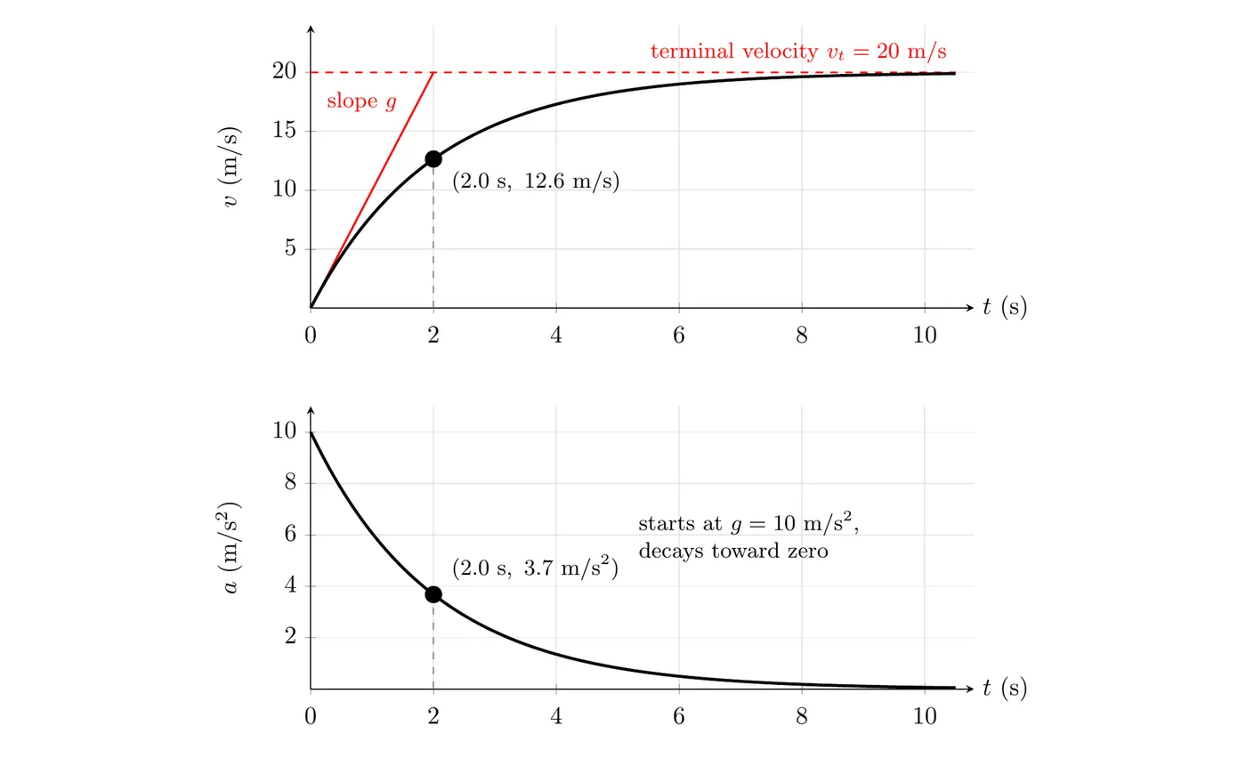
In the velocity graph, the red tangent line at

t = 0

has slope

g

and reaches

v_t

at exactly

t = \tau

. That’s a quick way to read the time constant off a graph.

Example Problem: Coasting With Only Drag

Change the forces and the asymptotes change. If there’s no constant force, only drag, the object just slows down. A 200 kg motorboat moving at 6.0 m/s cuts its engine and coasts, with water resistance

F_r = -kv

k = 50

kg/s.

DRAW and SUM: horizontally, drag is the only force, so

m\frac{dv}{dt} = -kv

SOLVE: separate the variables and integrate from the initial speed

v_0

t = 0

\int_{v_0}^{v} \frac{dv}{v} = -\frac{k}{m}\int_0^t dt \implies \ln\frac{v}{v_0} = -\frac{kt}{m} \implies v(t) = v_0 e^{-\frac{kt}{m}}

Integrate again (starting from

x = 0

) to get the position:

x(t) = \int_0^t v_0 e^{-\frac{kt'}{m}} dt' = \frac{mv_0}{k}\left(1 - e^{-\frac{kt}{m}}\right)

With the numbers,

\tau = \frac{m}{k} = \frac{200}{50} = 4.0

At $t = 4.0$ s, $v = 6.0e^{-1} = 2.2$ m/s and $x = 24\left(1 - e^{-1}\right) = 15.2$ m.

As $t \to \infty$ , $v \to 0$ , and the boat glides to a stop at $x_{max} = \frac{mv_0}{k} = \frac{(200)(6.0)}{50} = 24$ m.

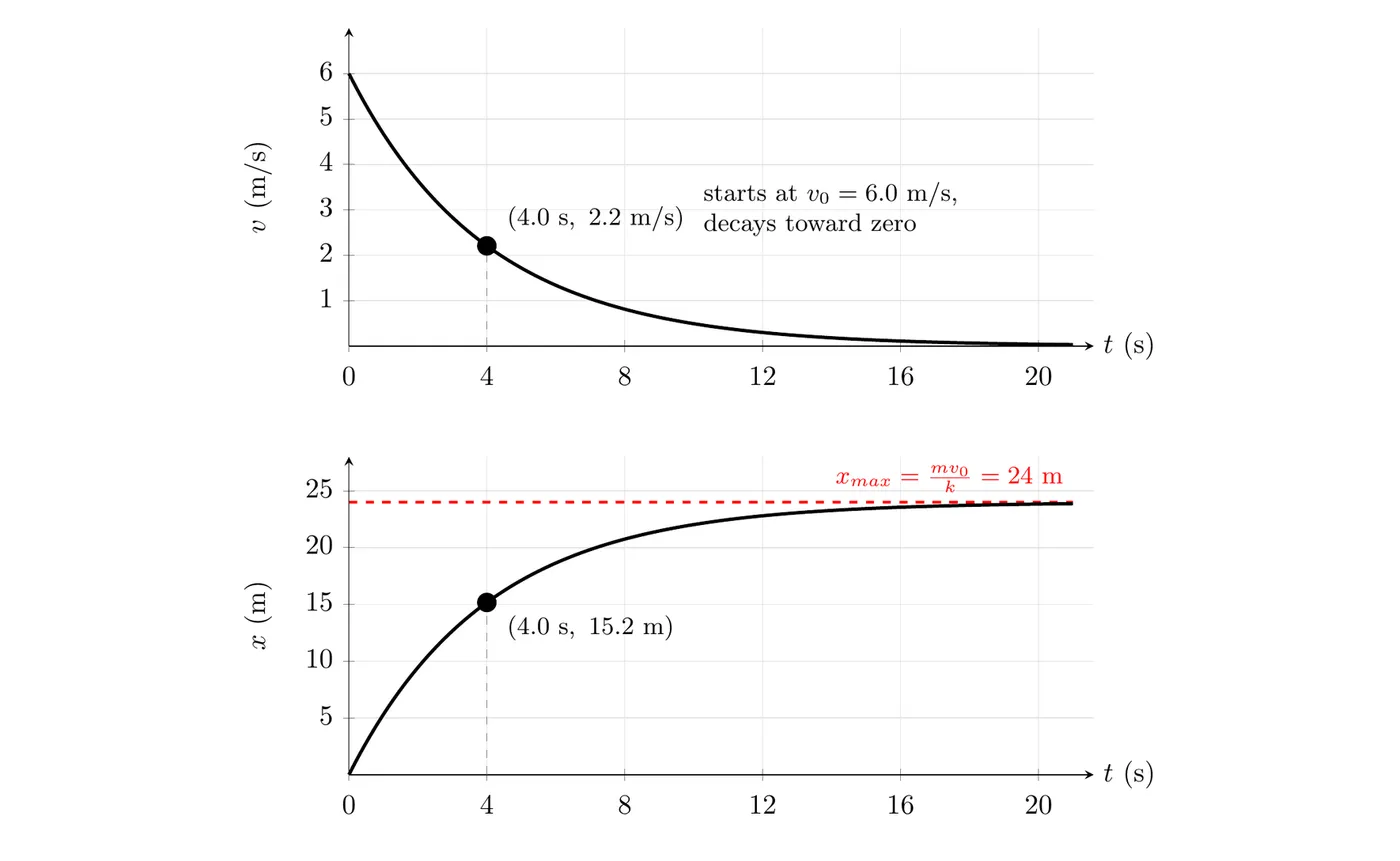
Here the velocity heads to zero (no force keeps the boat going) and the position heads to a fixed distance set by the starting speed. In this model the boat never quite stops, but it only covers a finite distance.

Key Mathematical Techniques Required

1. Separation of Variables

Get everything with one variable on one side and everything with the other variable on the other side.

2. Integration of Rational Functions

\int \frac{dx}{a + bx} = \frac{1}{b}\ln|a + bx| + C

3. Logarithm Properties

\ln(a) - \ln(b) = \ln\left(\frac{a}{b}\right)

\ln(a) + \ln(b) = \ln(ab)

4. The Exponential and Logarithm Relationship

\text{If } \ln(y) = x, \text{ then } y = e^x

5. Solving for Variables in Exponential Equations

Isolate the logarithm first, then exponentiate both sides.

Common Mistakes

Not spotting when to write a differential equation. Any time you see $\frac{dv}{dt}$ or $\frac{dx}{dt}$ in an equation, it’s a differential equation. For Part B you DON’T solve it, you just write it.

Dropping the negative sign in the resistive force. The force always opposes motion: $F_r = -kv$ , not $F_r = kv$ . That said, once you pick a positive direction and set up your equation, be careful with the signs.

Separating variables wrong. Make sure every $v$ term (including $dv$ ) is on one side and every $t$ term (including $dt$ ) is on the other before you integrate.

Natural log integration errors. The integral of $\frac{1}{a - bx}$ is $-\frac{1}{b}\ln|a - bx|$ , not $\frac{1}{b}\ln|a - bx|$ . Don’t lose the negative sign from the chain rule.

Forgetting the limits of integration. For definite integrals, use the right limits, usually 0 to $v(t)$ for velocity and 0 to $t$ for time.

Logarithm property errors. $\ln(a) - \ln(b) = \ln(\frac{a}{b})$ , NOT $\ln(a - b)$ . Brush up on the log rules before the exam.

Not simplifying with terminal velocity. On some problems you can sub in $v_t = \frac{mg}{k}$ to clean up your final answer.

Confusing terminal velocity with final velocity. Terminal velocity is the speed where drag balances gravity. The object approaches it forever but technically never quite gets there.

Sign errors when picking a positive direction. If down is positive, $F_g$ is positive and $F_r$ is negative. If up is positive, flip both. Stay consistent the whole way through.

Exponentiating wrong. When you have $\ln(f(v)) = g(t)$ , remember $f(v) = e^{g(t)}$ , not $f(v) = \ln^{-1}(g(t))$ .

Algebra slips when isolating v. After exponentiating, work through the algebra carefully to get $v$ by itself. People often botch a negative sign or mess up multiplying through by a constant.

Not checking the boundary conditions. Always test your solution at $t = 0$ (it should match the initial conditions) and as $t \to \infty$ (it should approach terminal velocity if there is one).

Back Next