2.1 - Tabular and Graphical Representations for the Distributions of Two Categorical Variables

Overview

In Unit 1 you summarized one categorical variable at a time. This topic looks at two categorical variables recorded on the same individuals, such as whether a person owns an e-reader and how many books they read last year. The big question is whether the variables are associated: does knowing someone's category for one variable tell you something about their category for the other? Two-way tables organize the counts, and side-by-side bar charts, segmented bar charts, and mosaic plots let you see the answer.

Two-way tables

A two-way table, also called a contingency table, summarizes data for two categorical variables. The categories (or levels) of one variable label the rows, the categories of the other label the columns, and each cell counts the individuals who fall in that row category and that column category at the same time.

Here is a survey of a random sample of 400 adults in a city. Each adult was asked whether they own an e-reader and how many books they read last year.

	0 books	1 to 5 books	6 or more books	Total
Owns an e-reader	12	48	60	120
No e-reader	84	140	56	280
Total	96	188	116	400

Cells: the six counts inside the table. The 48 means 48 adults own an e-reader and read 1 to 5 books.

Row totals: 120 adults own an e-reader and 280 do not.

Column totals: 96 read 0 books, 188 read 1 to 5, and 116 read 6 or more.

Grand total: 400 adults. The row totals and the column totals each add up to it ( $120 + 280 = 400$ and $96 + 188 + 116 = 400$ ), which is a quick check that you read the table right.

Counts or relative frequencies

The entries in a two-way table can be frequencies (counts) or relative frequencies (proportions or percents). A relative frequency is a count divided by a total. Which total you divide by changes the meaning completely, and Topic 2.2 goes through each choice.

To compare two groups, divide each cell by its group's total. Among the 120 e-reader owners, 60 read 6 or more books:

\frac{60}{120} = 0.50

So 50% of e-reader owners read 6 or more books last year. Doing this for every cell gives a table of percents within each row:

	0 books	1 to 5 books	6 or more books	Total
Owns an e-reader	10%	40%	50%	100%
No e-reader	30%	50%	20%	100%

Each row adds to 100% because each row is one complete group. When one variable naturally splits people into groups (here, owners and non-owners), compute percents within those groups and compare the other variable across them.

Graphs for two categorical variables

Every graph in this topic does the same basic job: for each category of one variable, it shows the frequency or relative frequency of each category of the other variable. They differ in what the bar heights and widths mean.

Side-by-side bar charts

A side-by-side bar chart (or clustered bar chart) draws a group of bars for each category of one variable, with one bar for each category of the other variable. Topic 1.4 used it to compare data sets; here the categories of the second variable play the role of the data sets. The bars can show counts or percents.

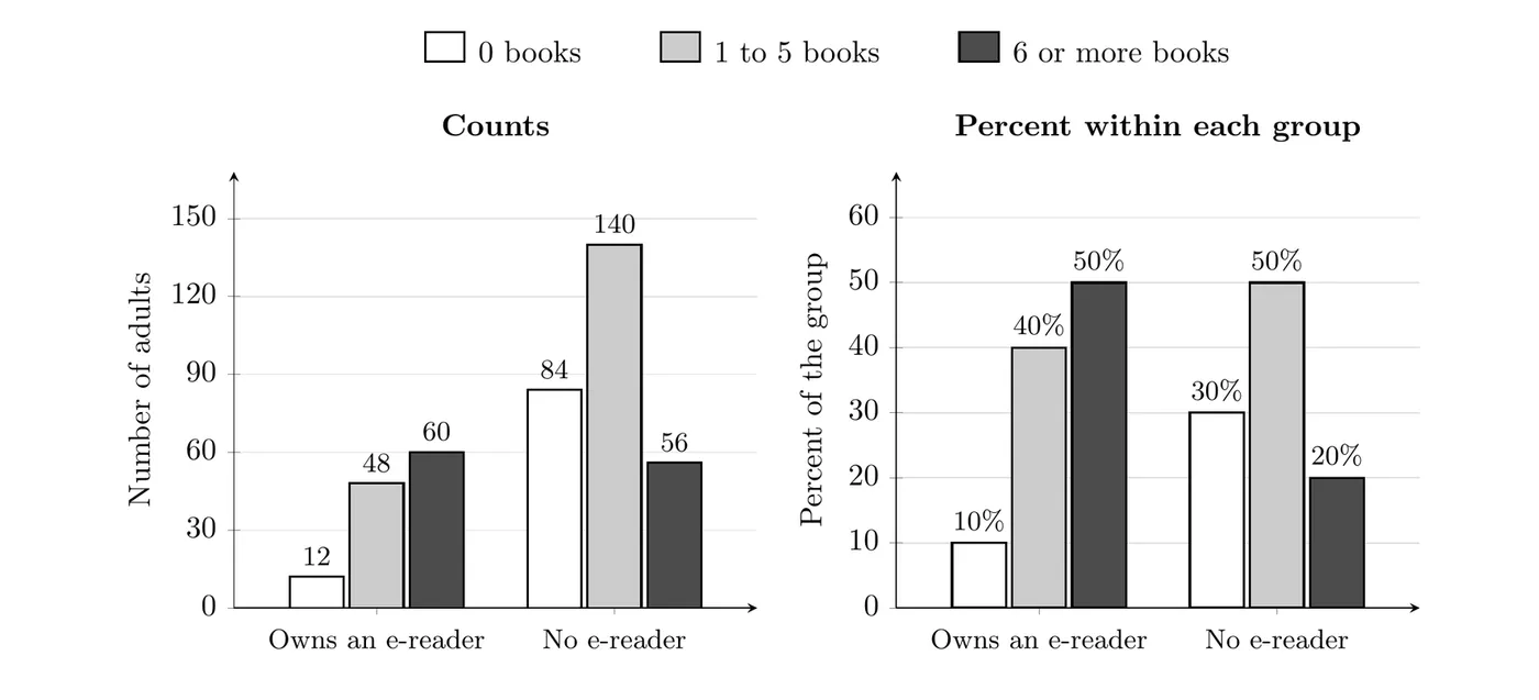
2.1 - Tabular and Graphical Representations for the Distributions of Two Categorical Variables

Look at the 6 or more books bars. In the counts panel they are almost the same height (60 and 56), which makes it seem like owners and non-owners read about the same. That's misleading, because there are more than twice as many non-owners (280) as owners (120). The percents panel fixes this: 50% of owners read 6 or more books, compared with only 20% of non-owners.

Rule of thumb: when the groups have different sizes, compare relative frequencies, not counts.

Segmented bar charts

A segmented bar chart (or stacked bar chart) draws one bar per group. Every bar is 100% tall and is split into segments, one for each category of the other variable. Each segment's height is the percent of that group in that category.

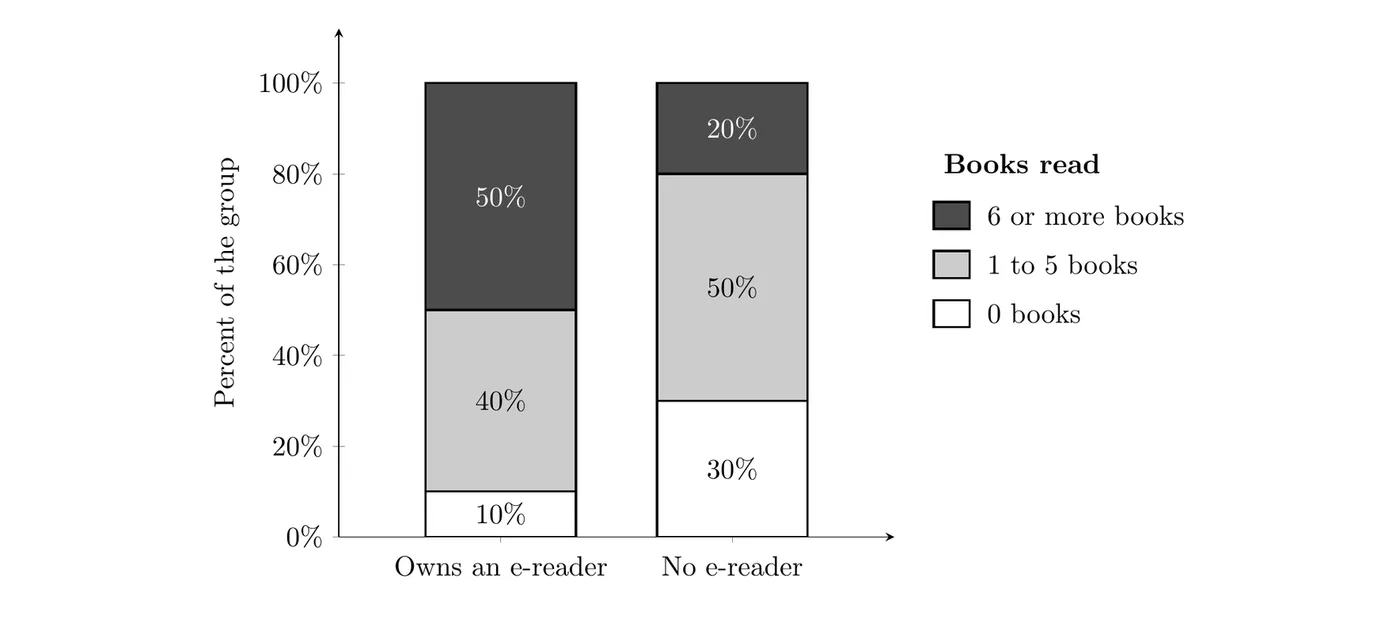
To read it, compare the same segment across bars. The dark segment (6 or more books) takes up 50% of the owners' bar but only 20% of the non-owners' bar. The white segment (0 books) is 10% for owners and 30% for non-owners. Segmented bar charts make whole distributions easy to compare, but because every bar is the same height, they hide how big each group is.

Mosaic plots

A mosaic plot is a segmented bar chart where each bar's width is proportional to the size of its group. Owners are

120/400 = 30\%

of the sample, so their column takes up 30% of the total width, and non-owners take up the other 70%.

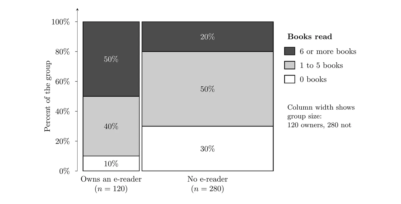
The heights inside each column are the same percents as the segmented bar chart, and the area of each tile is proportional to the count in that cell. A mosaic plot shows the group sizes and the distribution within each group in one picture.

Graph	What the bars show	Shows group sizes?	Best for
Side-by-side bar chart (counts)	Count in each cell	Yes	Groups of about the same size
Side-by-side bar chart (percents)	Percent within each group	No	Comparing groups one category at a time
Segmented bar chart	Percent within each group, bars total 100%	No	Comparing whole distributions
Mosaic plot	Percent within each group, width = group size	Yes	Seeing distributions and group sizes together

Seeing an association

Two categorical variables are associated if the distribution of one variable is different for different categories of the other variable. In a segmented bar chart or mosaic plot, that means the segments change from bar to bar. If the bars look the same, there is no association.

What would no association look like here? Then owners and non-owners would read books at the same rates, and both groups would match the 400 adults overall:

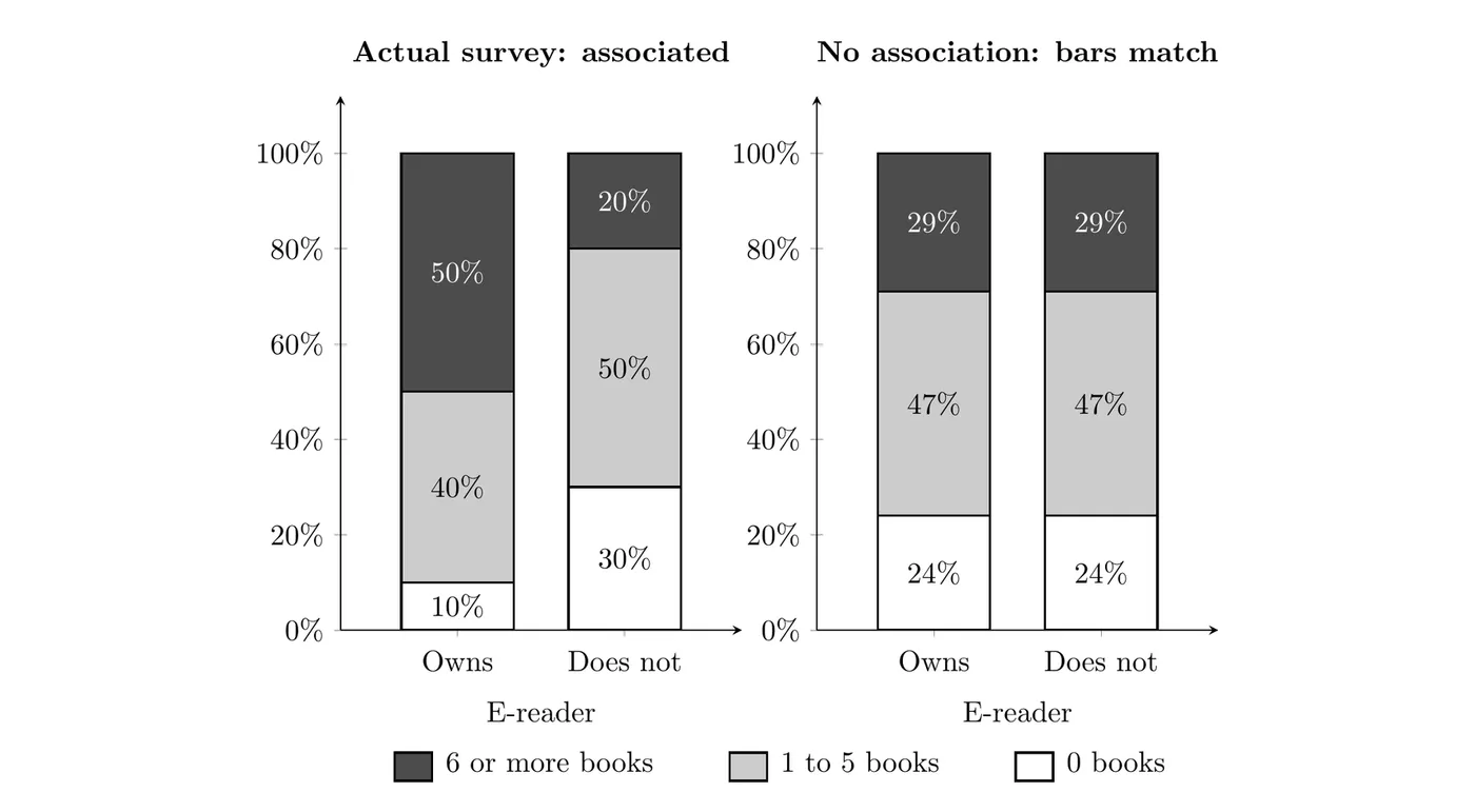
\frac{96}{400} = 0.24 \qquad \frac{188}{400} = 0.47 \qquad \frac{116}{400} = 0.29

The actual bars (left) are very different from each other, while the no-association bars (right) match exactly. So e-reader ownership and number of books read are associated for these adults: owners tend to read more books.

Association works both ways. If reading differs by ownership, then ownership also differs by reading. Among adults who read 0 books, only $12/96 = 0.125$ own an e-reader, while among adults who read 6 or more books, $60/116 \approx 0.517$ do.

Association is not causation. This is a survey, so it can't show that owning an e-reader makes people read more. People who already love reading may be the ones who buy e-readers.

Small differences can happen by chance. In sample data, a big difference like 50% vs. 20% is convincing, but a small one like 50% vs. 48% could show up even if there were no association in the population. The chi-square test in Unit 3 makes this call precise.

Justifying claims with tables and graphs

AP questions often give a table or graph and ask whether it supports a claim. A complete answer does three things:

Quote specific values from each group being compared (percents or proportions, not just "the bar is taller").

Compare them directly: which is larger, and by about how much.

Conclude in context, using the names of the variables and the people or things studied.

Weak answer: "The bars are different, so the claim is true."

Strong answer: "50% of the e-reader owners read 6 or more books last year, compared with only 20% of the adults without an e-reader. Since frequent readers make up a much larger share of owners, the data support the claim that e-reader ownership and the number of books read are associated for adults in this city."

Example 1: Snacks at the movies

A movie theater surveyed 200 customers about their age group and the snack they bought.

	Popcorn	Candy	No snack	Total
Under 30	40	24	16	80
30 and older	48	12	60	120
Total	88	36	76	200

(a) How many customers were 30 and older and bought candy?

Read the cell in the "30 and older" row and "Candy" column: 12 customers.

(b) Find the distribution of snack choice within each age group.

Divide each cell by its row total:

\text{Under 30: } \frac{40}{80} = 0.50, \quad \frac{24}{80} = 0.30, \quad \frac{16}{80} = 0.20

\text{30 and older: } \frac{48}{120} = 0.40, \quad \frac{12}{120} = 0.10, \quad \frac{60}{120} = 0.50

Among customers under 30, 50% bought popcorn, 30% bought candy, and 20% bought no snack. Among customers 30 and older, 40% bought popcorn, 10% bought candy, and 50% bought no snack. The distributions are clearly different, so age group and snack choice are associated for these customers.

(c) The manager says, "More customers 30 and older bought popcorn than customers under 30, so older customers are more likely to buy popcorn." Do the data support this?

No. It's true that more older customers bought popcorn (48 vs. 40), but there were more older customers to begin with (120 vs. 80). As a proportion of each group, 50% of customers under 30 bought popcorn compared with 40% of customers 30 and older. Younger customers were more likely to buy popcorn, so the manager's claim is not supported.

Example 2: Part-time jobs by grade (AP-style)

A high school asked all 500 of its students whether they have a part-time job. The mosaic plot shows the results by grade level.

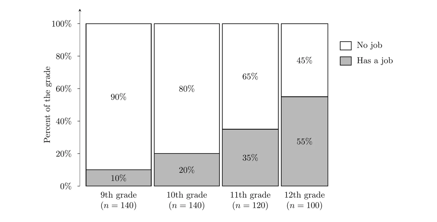
(a) What do the widths of the columns tell you?

The width of each column is proportional to the number of students in that grade. The 9th and 10th grade columns are the widest (140 students each), then 11th grade (120), and 12th grade is the narrowest (100).

(b) Is there an association between grade level and having a part-time job? Justify your answer.

Yes. The percent of students with a job rises with each grade: 10% of 9th graders, 20% of 10th graders, 35% of 11th graders, and 55% of 12th graders. The distribution of job status is different for every grade level, so grade level and having a part-time job are associated for the students at this school.

(c) A student says, "Most students who have a job are seniors." Is that correct?

Convert each percent back to a count by multiplying by the grade's size:

0.10(140) = 14 \qquad 0.20(140) = 28 \qquad 0.35(120) = 42 \qquad 0.55(100) = 55

That's

14 + 28 + 42 + 55 = 139

students with jobs, and the proportion who are seniors is

\frac{55}{139} \approx 0.396

So only about 40% of the students with jobs are seniors, not most of them. The claim mixes up "55% of seniors have a job" with "55% of students with jobs are seniors." These answer different questions, and Topic 2.2 shows how to tell them apart.

Common mistakes

Comparing counts when the groups have different sizes. Compare percents within each group instead.

Mixing up the direction of a percent. "Percent of seniors who have a job" and "percent of students with a job who are seniors" use different groups and give different answers.

Saying "they're associated" without numbers. Quote values from each group and compare them.

Claiming cause and effect from a survey. An association in observational data does not show that one variable causes the other.

Expecting a segmented bar chart to show group sizes. Every bar is 100% tall. Use the table or a mosaic plot for group sizes.

Back Next