2.9 - Parameters of Random Variables

Overview

A probability distribution (Topic 2.8) lists every value a random variable can take and how likely each one is. That's a lot of information, so we summarize it with two numbers: the mean (also called the expected value), which describes the center, and the standard deviation, which describes how much the values typically vary. This topic covers how to calculate both for a discrete random variable and, just as important, how to interpret them in context.

Parameters

A parameter is a number that describes a characteristic of a probability distribution of a random variable, or of a population. The mean and standard deviation of a random variable are both parameters.

The key fact: the value of a parameter is a single, fixed value. It doesn't change from one observation to the next. A statistic is different: it's calculated from a sample, so it changes from sample to sample. The symbols are the ones from Topic 1.2 (

\mu

and

\sigma

for parameters,

\bar{x}

and

s

for statistics). For a random variable

X

, the parameters are often written

\mu_X

and

\sigma_X

The expected value (mean)

The expected value, or mean, of a random variable

X

is written

E(X)

\mu_X

. For a discrete random variable:

\mu_X = E(X) = \sum x_i \cdot P(x_i)

Here

x_i

is each possible value of the random variable and

P(x_i)

is the probability of that value. In words: multiply each value by its probability, then add up the products. This formula is on the AP formula sheet.

A discrete random variable can only take on values that are countable or finite, like 0, 1, 2, 3. The number of tacos someone orders, the number of heads in 10 flips, and the number of defective phones in a shipment are all discrete. (Variables that can take any value in an interval, like height or time, are continuous. They come in Topic 2.11.)

Why the formula works

The expected value is a weighted average. Each value counts in proportion to its probability, so likely values pull the mean toward them more than unlikely ones. If every value were equally likely, it would just be the ordinary average of the values.

On a probability histogram, the mean is the balance point. If the bars were blocks sitting on a seesaw, the seesaw would balance at

\mu_X

Interpreting the expected value

The expected value is the long-run average outcome of the random variable. If the random process were repeated many, many times, the average of all the values of

X

would get closer and closer to

\mu_X

The expected value isn't a prediction for any one trial, and it doesn't have to be a value

X

can actually take. No customer orders 2.5 tacos, but the mean number of tacos per customer can still be 2.5.

Example 1: Expected number of tacos

Use the taco truck distribution from Topic 2.8, where

X

= the number of tacos ordered by a randomly selected customer (Example 1 there found the missing value,

P(X = 4) = 0.15

). Calculate

E(X)

and interpret it in context.

Step 1: Multiply each value by its probability. A third row keeps the work organized.

$x$	1	2	3	4	5	Total
$P(x)$	0.20	0.35	0.25	0.15	0.05	1.00
$x \cdot P(x)$	0.20	0.70	0.75	0.60	0.25	2.50

Step 2: Add the products.

\mu_X = 1(0.20) + 2(0.35) + 3(0.25) + 4(0.15) + 5(0.05) = 2.5

Answer:

E(X) = 2.5

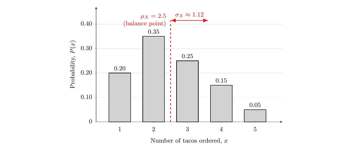
tacos. If we randomly selected many, many customers at this taco truck, the average number of tacos ordered per customer would be about 2.5 tacos.

Standard deviation and variance

The standard deviation of a random variable, written

SD(X)

\sigma_X

, measures how far the values of

X

typically fall from the mean. For a discrete random variable:

\sigma_X = \sqrt{\sum (x_i - \mu_X)^2 \cdot P(x_i)}

This is also on the formula sheet. To use it:

Find the mean $\mu_X$ first.

For each value, find its deviation from the mean, $x_i - \mu_X$ , and square it.

Multiply each squared deviation by its probability.

Add these products. The sum is the variance.

Take the square root to get the standard deviation.

The variance of a random variable is the square of its standard deviation, written

V(X)

\sigma_X^2

\sigma_X^2 = V(X) = \sum (x_i - \mu_X)^2 \cdot P(x_i)

Why square, then take a root? Deviations above the mean are positive and deviations below are negative. Weighted by their probabilities, they always add to exactly 0, so they'd tell you nothing. Squaring makes every deviation positive. The catch is that variance is in squared units ("tacos squared"), which is hard to picture. The square root puts the standard deviation back in the original units, so that's the number we usually report.

Interpreting the standard deviation

The standard deviation is the typical distance between the values of the random variable and its mean, over the long run. A small

\sigma_X

means outcomes usually land close to the mean. A large

\sigma_X

means they're often far from it.

Example 2: Standard deviation of tacos

Calculate and interpret

\sigma_X

for the taco distribution in Example 1, where

\mu_X = 2.5

Step 1: Find each squared deviation and weight it by its probability.

$x$	$P(x)$	$x - \mu_X$	$(x - \mu_X)^2$	$(x - \mu_X)^2 \cdot P(x)$
1	0.20	$-1.5$	2.25	0.4500
2	0.35	$-0.5$	0.25	0.0875
3	0.25	0.5	0.25	0.0625
4	0.15	1.5	2.25	0.3375
5	0.05	2.5	6.25	0.3125

Step 2: Add to get the variance.

\sigma_X^2 = 0.4500 + 0.0875 + 0.0625 + 0.3375 + 0.3125 = 1.25

Step 3: Take the square root.

\sigma_X = \sqrt{1.25} \approx 1.12

Answer:

\sigma_X \approx 1.12

tacos. Over many, many randomly selected customers at this taco truck, the number of tacos a customer orders typically varies by about 1.12 tacos from the mean of 2.5 tacos.

On the TI-84

Enter the values of

X

in L1 and the probabilities in L2 (STAT, EDIT). Then run STAT, CALC, 1-Var Stats with List: L1 and FreqList: L2. The output labeled

\bar{x}

\mu_X

, and

\sigma x

\sigma_X

. This is a good way to check your work, but on the AP exam you still need to show the formula with the numbers substituted in. A calculator result alone doesn't show your method.

Interpreting parameters in context

The AP exam expects the mean and standard deviation of a random variable to be interpreted in the context of a specific population. A bare number like "the mean is 2.5" earns no credit. A complete interpretation names the variable in context, gives the units, and uses the long-run idea.

Mean: "If we [repeat the random process] many, many times, the average [variable in context] will be about $\mu_X$ [units]."

Standard deviation: "The [variable in context] will typically vary by about $\sigma_X$ [units] from the mean of $\mu_X$ [units]."

Name the population you're describing: "customers at this taco truck," not "people." The distribution came from that taco truck's records, so the parameters describe that taco truck.

Example 3: Same mean, different spread

Suppose the delivery time (in days) for a package shipped by Company A or Company B has these distributions.

Delivery time (days)	1	2	3	4	5
Company A probability	0	0.2	0.6	0.2	0
Company B probability	0.2	0.2	0.2	0.2	0.2

Compare the two companies using the mean and standard deviation of delivery time.

Means:

\mu_A = 2(0.2) + 3(0.6) + 4(0.2) = 3 \qquad \mu_B = (1 + 2 + 3 + 4 + 5)(0.2) = 3

Standard deviations:

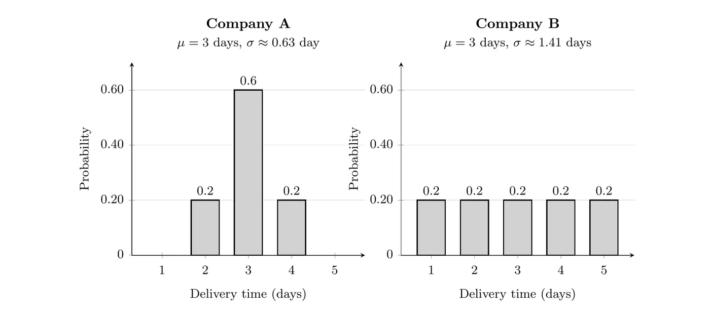
\sigma_A = \sqrt{(2-3)^2(0.2) + (3-3)^2(0.6) + (4-3)^2(0.2)} = \sqrt{0.4} \approx 0.63

\sigma_B = \sqrt{\left[(1-3)^2 + (2-3)^2 + (3-3)^2 + (4-3)^2 + (5-3)^2\right](0.2)} = \sqrt{10(0.2)} = \sqrt{2} \approx 1.41

Answer: Over many, many packages, both companies average 3 days per delivery. But Company A's delivery times typically vary by about 0.63 day from 3 days, while Company B's typically vary by about 1.41 days from 3 days. If a package has to arrive by a deadline, Company A is the more predictable choice. The mean alone would have hidden that difference.

Example 4: Is the raffle worth it? (AP-style)

A school sells 500 raffle tickets for $5 each. One ticket wins $500, two tickets win $100 each, and five tickets win $20 each. The other tickets win nothing. You buy one ticket. Let

X

= your net gain, the prize minus the $5 you paid.

(a) Construct the probability distribution of

X

. (b) Calculate and interpret

E(X)

. (c) Calculate and interpret

\sigma_X

. (d) Use

E(X)

to explain how the raffle helps the school.

(a) Subtract the $5 ticket price from each prize. Each probability is the number of tickets with that prize out of 500.

Net gain $x$	$495	$95	$15	$-$ $5
$P(x)$	$\frac{1}{500} = 0.002$	$\frac{2}{500} = 0.004$	$\frac{5}{500} = 0.010$	$\frac{492}{500} = 0.984$

The probabilities add to

0.002 + 0.004 + 0.010 + 0.984 = 1

, as they should.

(b)

E(X) = 495(0.002) + 95(0.004) + 15(0.010) + (-5)(0.984) = 0.99 + 0.38 + 0.15 - 4.92 = -3.40

If you bought a ticket in many, many raffles just like this one, your average net gain would be about

-

$3.40 per ticket. In other words, you'd lose about $3.40 per ticket in the long run.

(c)

First the variance, using

\mu_X = -3.40

\begin{aligned} \sigma_X^2 &= (495 - (-3.40))^2(0.002) + (95 - (-3.40))^2(0.004) \\ &\quad + (15 - (-3.40))^2(0.010) + (-5 - (-3.40))^2(0.984) \\ &\approx 496.805 + 38.730 + 3.386 + 2.519 = 541.44 \end{aligned}

\sigma_X = \sqrt{541.44} \approx 23.27

Over many, many tickets in raffles like this one, a ticket's net gain typically varies by about $23.27 from the mean of

-

$3.40. The standard deviation is large compared with the mean because of the rare $495 win.

(d) Buyers lose $3.40 per ticket on average, so the school gains $3.40 per ticket on average. Selling all 500 tickets, the school raises

500 \times \$3.40 = \$1{,}700

. That matches a direct count: ticket sales bring in

500 \times \$5 = \$2{,}500

, and the prizes cost

\$500 + 2(\$100) + 5(\$20) = \$800

, so the school keeps

\$2{,}500 - \$800 = \$1{,}700

Side note: the expected prize per ticket is

\$800 / 500 = \$1.60

. A ticket priced at $1.60 would make

E(X) = 0

, which is called a fair game. Any higher price means buyers lose money in the long run.

Common mistakes

Averaging the values instead of weighting them. For the taco distribution, $(1 + 2 + 3 + 4 + 5)/5 = 3$ is not the mean. Multiply each value by its probability.

Forgetting the square root. $\sum (x_i - \mu_X)^2 \cdot P(x_i)$ is the variance, not the standard deviation.

Treating the expected value as a prediction. $E(X) = 2.5$ tacos doesn't mean the next customer orders 2 or 3 tacos. It's a long-run average over many customers.

Interpreting without context or units. Say what the variable is, the units, and the population: "tacos per customer at this taco truck."

Not checking that the probabilities add to 1. If they don't, a value is missing or a probability is wrong.

Mixing up parameters and statistics. $\mu_X = 2.5$ is fixed. The average number of tacos for the 20 customers you watched today is a statistic, and it changes from day to day.

Back Next