2.12 - Sampling Distributions and the Central Limit Theorem

Overview

When you take a random sample and calculate a statistic, like the sample mean

\bar{x}

, you get one number. A different random sample would give a different number. A sampling distribution describes how a statistic varies from sample to sample. It's the bridge between probability and inference: in Units 3 and 4, sampling distributions tell you how far a statistic is likely to land from the parameter it estimates. This topic covers what a sampling distribution is, how to approximate one with a simulation, randomization distributions for experiments, and the central limit theorem.

Three different distributions

Students lose points on the AP exam by mixing up three kinds of distributions. Be specific about which one you mean.

Distribution	What it shows	Example: wait times at a clinic
Population distribution	the values of a variable for every individual in the population	the wait times of all patients
Distribution of sample data	the values for the individuals in one sample	the wait times of the 30 patients in your sample
Sampling distribution of a statistic	the values of a statistic, like $\bar{x}$ , from all possible samples of the same size	the mean wait time $\bar{x}$ for every possible sample of 30 patients

The first two show individuals. A sampling distribution shows statistics, one value per sample.

Watch your wording. "Larger samples have less variability" is ambiguous. It's false about the sample data: a bigger sample's values are just as spread out as the population's. It's true about the sampling distribution: sample means from larger samples vary less from sample to sample. Say "the sampling distribution of

\bar{x}

is less variable when

n

is larger," and avoid using "it" when it could mean more than one distribution.

What a sampling distribution is

A sampling distribution of a statistic is the distribution of values of the statistic for all possible samples of a given size from a given population. Real populations are too big to list every sample, but a tiny population shows the idea completely.

Example 1: Every possible sample

Five friends read 2, 4, 6, 8, and 10 books over the summer. Treat these five friends as the whole population, so the population mean is

\mu = \frac{2 + 4 + 6 + 8 + 10}{5} = 6

books. Find the sampling distribution of

\bar{x}

for random samples of 2 friends (without replacement).

Step 1: List every possible sample. There are

\binom{5}{2} = 10

samples of size 2.

Sample	2, 4	2, 6	2, 8	2, 10	4, 6	4, 8	4, 10	6, 8	6, 10	8, 10
$\bar{x}$	3	4	5	6	5	6	7	7	8	9

Step 2: Make the distribution of the sample means. Each sample is equally likely, so each has probability

\frac{1}{10}

$\bar{x}$	3	4	5	6	7	8	9
Probability	0.1	0.1	0.2	0.2	0.2	0.1	0.1

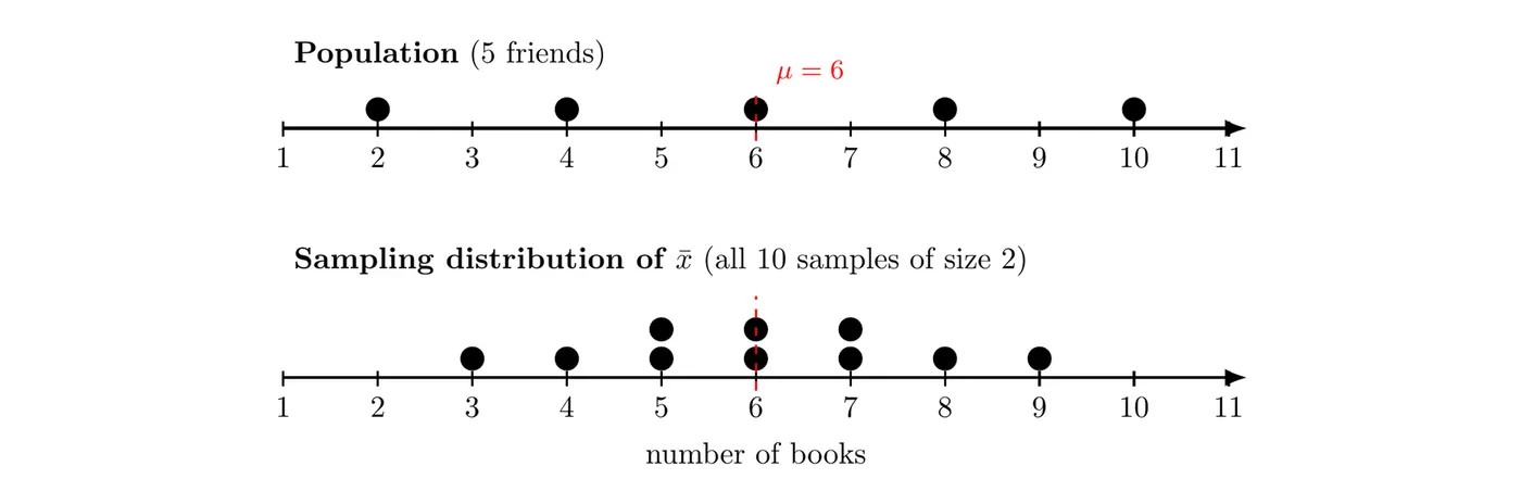
2.12 - Sampling Distributions and the Central Limit Theorem

What it shows:

Center: the mean of all 10 sample means is $\frac{3 + 4 + 5 + 5 + 6 + 6 + 7 + 7 + 8 + 9}{10} = 6$ , exactly $\mu$ . Sample means don't systematically miss high or low.

Variability: the sample means run from 3 to 9, while the population runs from 2 to 10. Averaging two values pulls extreme values toward the middle. The population's standard deviation is about 2.83 books, but the sample means' standard deviation is only about 1.73 books.

Sampling variability: most samples give an $\bar{x}$ that isn't 6. Different samples give different statistics. That isn't a mistake. It's the nature of sampling.

Simulating a sampling distribution

When there are too many possible samples to list, simulate. Assume known values for the population parameters, then:

Use technology to generate a random sample of size $n$ from the population.

Calculate the statistic for that sample and record it.

Repeat many times (hundreds or thousands).

Graph the recorded values. This distribution of simulated statistics approximates the sampling distribution of the statistic.

Describe a simulated sampling distribution the same way you'd describe any distribution: shape, center, and variability, in context.

Example 2: Simulated sample means

Suppose the wait times at a clinic are strongly skewed right, with mean

\mu = 10

minutes and standard deviation

\sigma = 10

minutes. Most waits are short, but a few are very long. A computer took 2,000 random samples of each size

n = 2

n = 10

, and

n = 30

from this population and recorded

\bar{x}

for each sample. The red curves are normal curves with the same mean and standard deviation as the simulated sample means.

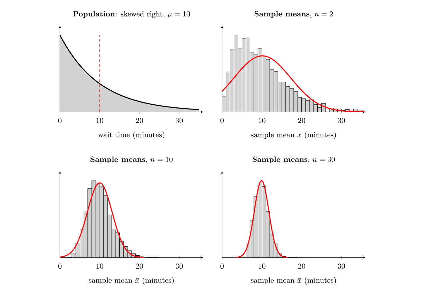
Describe how the sampling distribution of

\bar{x}

changes as

n

increases.

Shape: for $n = 2$ , the sample means are still clearly skewed right, and the normal curve fits badly. For $n = 10$ , they're only slightly skewed. For $n = 30$ , they're approximately normal.

Center: all three are centered close to the population mean of 10 minutes. The simulated means of the $\bar{x}$ values were 10.11, 10.01, and 9.92 minutes.

Variability: the standard deviation of the sample means shrinks as $n$ grows: about 7.15, 3.12, and 1.82 minutes. Means of larger samples land closer to $\mu$ more consistently.

Topic 4.1 gives the formula behind that shrinking spread,

\sigma_{\bar{x}} = \frac{\sigma}{\sqrt{n}}

. For

n = 30

, it gives

\frac{10}{\sqrt{30}} \approx 1.83

minutes, which matches the simulation.

Randomization distributions

In an experiment, the randomness comes from random assignment of treatments, not from random sampling. A randomization distribution is the distribution of a statistic generated by simulation from repeatedly reallocating (reassigning) the response values to the treatment groups at random. For each reallocation, calculate and record the statistic. The resulting distribution approximates the sampling distribution of the statistic when the treatment has no effect.

The logic: if the treatment does nothing, each subject's response would have been the same no matter which group it was in. Shuffling the responses into new groups shows how big a difference random assignment alone tends to create.

Example 3: Fertilizer and plant growth

A student randomly assigns 12 bean seedlings to two groups of 6. One group gets a new fertilizer, and the other gets plain water. Here are the heights after three weeks.

Group	Heights (cm)	Mean (cm)
Fertilizer	14.2, 15.1, 13.6, 15.8, 14.9, 14.0	14.6
Water	13.4, 12.8, 14.3, 14.1, 13.1, 14.5	13.7

The observed difference in means is

\bar{x}_F - \bar{x}_W = 14.6 - 13.7 = 0.90

cm. Is that big, or could random assignment alone produce it?

Step 1: Reallocate. Write the 12 heights on cards, shuffle, deal 6 to "fertilizer" and 6 to "water," and calculate the difference in means.

Step 2: Repeat. The dotplot shows 200 reallocations done by computer.

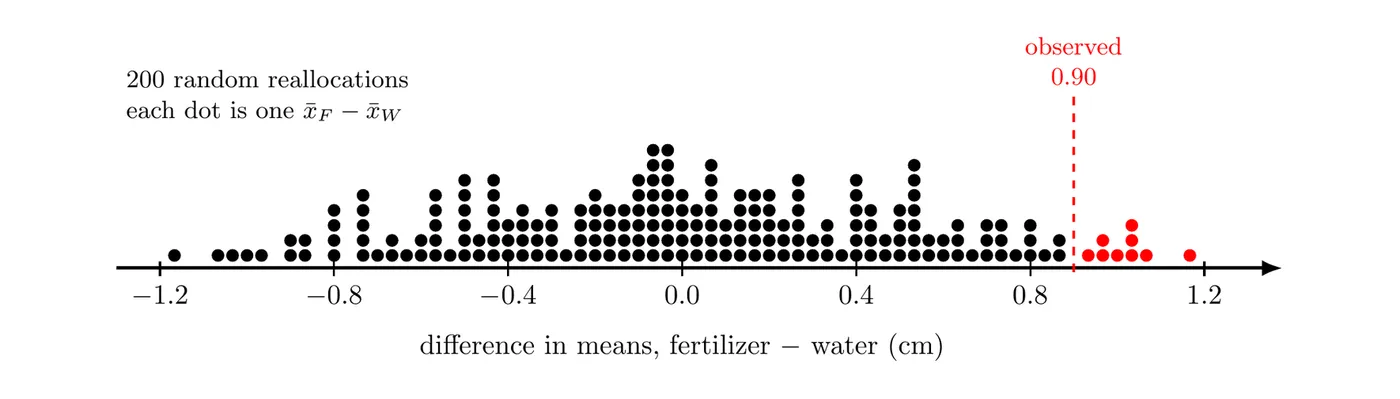
Step 3: Describe and compare. The randomization distribution is roughly symmetric and centered at about 0 cm, which makes sense: shuffling assumes the fertilizer has no effect. Most differences fall between about

-1

and

1

cm. Only 9 of the 200 reallocations (4.5%) gave a difference of 0.90 cm or more.

Answer: a difference as large as the observed 0.90 cm is unusual when random assignment is the only thing at work. Because the seedlings were randomly assigned, this is evidence that the fertilizer helps them grow taller. Later in the course you'll make this kind of reasoning formal with significance tests.

The central limit theorem

The central limit theorem (CLT) states that the sampling distribution of the mean of a random sample has a shape that can be approximated by a normal distribution. The larger the sample, the better the approximation. Example 2 shows it happening: the population of wait times is strongly skewed, yet the sample means for

n = 30

are approximately normal.

It works for any population shape, as long as the sample is random and large enough. How large depends on the population. The more skewed the population, the larger $n$ needs to be. The usual guideline in AP Statistics is $n \ge 30$ , and an extremely skewed population may need more.

If the population is normal, the sampling distribution of $\bar{x}$ is normal for any sample size, even $n = 2$ . The CLT matters when the population isn't normal.

The CLT is about the sampling distribution of the sample mean. It's not about the population or the data in one sample. A random sample of 100 wait times will still look skewed right, because sample data look like the population they came from.

Why it matters: once you know $\bar{x}$ is approximately normal, you can use the normal calculations from Topic 2.11 to find probabilities about sample means. That's the foundation for inference about means in Unit 4.

Example 4: Which distribution is approximately normal? (AP-style)

The amount customers spend per visit at a coffee shop is strongly skewed right, with mean $8.40 and standard deviation $6.10. A manager selects a random sample of 50 receipts.

(a) Describe the shape of the distribution of the 50 amounts in the sample. (b) Describe the shape of the sampling distribution of the sample mean amount,

\bar{x}

, for random samples of 50 receipts. (c) Would the sampling distribution of

\bar{x}

for random samples of 3 receipts be approximately normal? Explain.

(a) Most likely skewed right. A random sample tends to resemble the population it came from, and the population of amounts is strongly skewed right. The central limit theorem doesn't apply to the data in one sample.

(b) Approximately normal. By the central limit theorem, the sampling distribution of the mean of a random sample is approximately normal when the sample is large, and

n = 50 \ge 30

, even though the population is skewed right.

(c) No. With only

n = 3

receipts from a strongly skewed population, the sampling distribution of

\bar{x}

will still be noticeably skewed right, like the

n = 2

panel in Example 2.

Common mistakes

Mixing up the three distributions. Say "the sampling distribution of the sample mean," not "the distribution" or "it."

Saying the CLT makes the population or the sample normal. It only describes the sampling distribution of $\bar{x}$ .

Writing "larger samples have less variability." Say which distribution: the sampling distribution of $\bar{x}$ is less variable for larger samples.

Expecting a simulation to be centered at the observed statistic. A simulated sampling distribution is centered near the assumed parameter, and a randomization distribution of a difference is centered near 0. The observed statistic is what you compare to it.

Running too few repetitions. Ten simulated samples give a rough picture at best. Use hundreds.

Treating $n \ge 30$ as magic. With a normal population, any $n$ works. With an extremely skewed population, 30 may not be enough.

Back Next