2.11 - The Normal Distribution

Overview

So far, the random variables in this unit have been discrete: you could list their values. Many variables, like height, weight, and time, can take any value in a range. These are continuous, and the most important model for them is the normal distribution, the familiar bell curve. This topic covers what a normal distribution looks like, how its mean and standard deviation control its shape, the empirical rule, how to find probabilities and cutoff values, and how to compare positions with percentiles.

Continuous random variables

A continuous random variable can take on any value within a specified domain, like any time between 0 and 60 minutes or any weight between 40 and 80 grams. Compare that with a discrete random variable, whose values you can count.

There are infinitely many possible values in an interval, so we can't list a probability for each one. Instead, every interval within the domain has a probability, given by the area under a curve over that interval. The total area under the curve is 1, just like the probabilities of a discrete distribution add to 1.

One consequence: the probability of any single exact value is 0, because a single point has no area. So for a continuous random variable,

P(X < 5) = P(X \le 5)

. That's different from the binomial distribution, where

<

and

\le

give different answers.

The normal distribution

Many continuous random variables are well modeled by a normal distribution: heights of adults, weights of eggs, errors in measurements, scores on many standardized tests. A normal curve is

continuous (a smooth curve with no gaps),

unimodal (one peak),

bell-shaped, and

symmetric about its mean, so the mean, median, and peak are all at the same place.

A normal curve can model a distribution of data, like a histogram of 1,000 people's heights, or a continuous random variable, like the weight of the next egg a farm produces.

Two parameters: the mean and the standard deviation

A normal distribution is completely identified by two parameters, its mean

\mu

and its standard deviation

\sigma

The mean sets the center. The peak and the line of symmetry are at $\mu$ . Changing $\mu$ slides the whole curve left or right without changing its shape.

The standard deviation sets the spread. The smaller the standard deviation, the taller and more concentrated the curve is around its mean. The larger the standard deviation, the shorter and less concentrated it is. The curve has to get shorter as it spreads out, because the total area stays 1.

You can see the standard deviation on the graph. The curve switches from concave down to concave up (its inflection points) exactly one standard deviation from the mean, at $\mu - \sigma$ and $\mu + \sigma$ .

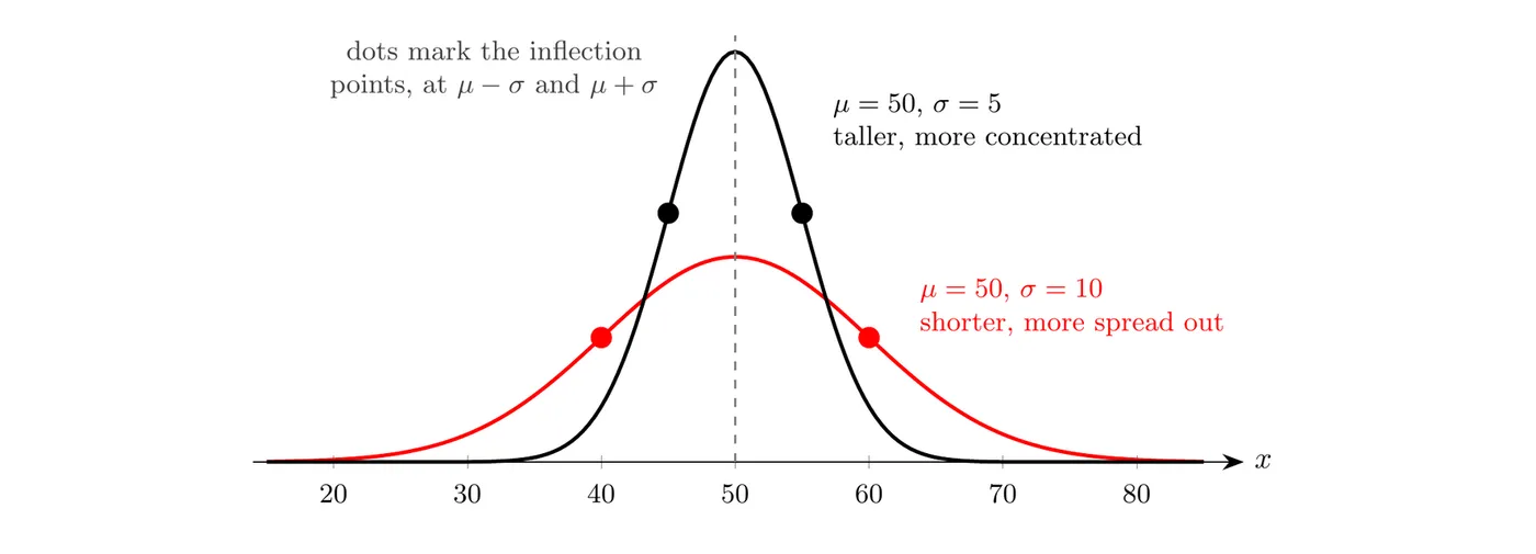
A common shorthand is

N(\mu, \sigma)

. For example,

N(50, 5)

is the normal distribution with mean 50 and standard deviation 5.

The standard normal distribution

The standard normal distribution is the normal distribution with mean

\mu = 0

and standard deviation

\sigma = 1

, or

N(0, 1)

. Any normal distribution can be converted to the standard normal with

z

-scores (Topic 1.9):

z = \frac{x - \mu}{\sigma}

z

-score tells you how many standard deviations a value is above the mean (positive) or below it (negative). If

X

is normal, its

z

-scores follow the standard normal distribution, so one table works for every normal distribution. That table is Table A in the formulas and tables you get on the AP exam, and it gives the area to the left of each

z

-score.

The empirical rule

For any normal distribution:

about 68% of the values are within 1 standard deviation of the mean, between $\mu - \sigma$ and $\mu + \sigma$

about 95% are within 2 standard deviations, between $\mu - 2\sigma$ and $\mu + 2\sigma$ , and

about 99.7% are within 3 standard deviations, between $\mu - 3\sigma$ and $\mu + 3\sigma$ .

This is the empirical rule, also called the 68-95-99.7 rule. It estimates areas under a normal curve. Because the curve is symmetric, you can split the pieces in half: 34% between

\mu

and

\mu + \sigma

, 13.5% between

\mu + \sigma

and

\mu + 2\sigma

(half of

95 - 68

), 2.35% between

\mu + 2\sigma

and

\mu + 3\sigma

(half of

99.7 - 95

), and 0.15% beyond

\mu + 3\sigma

. The left side is the mirror image.

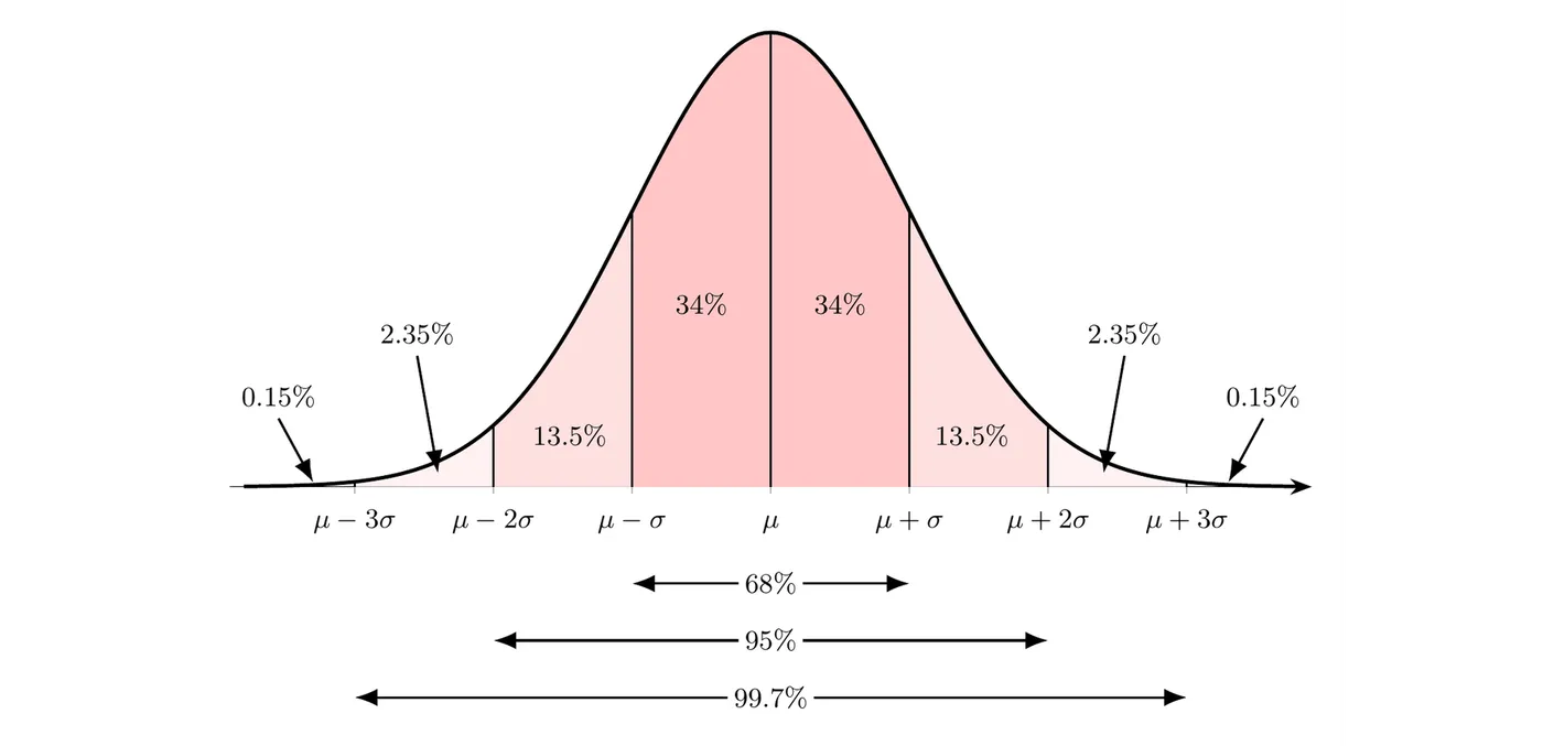
Use the empirical rule only for boundaries exactly 1, 2, or 3 standard deviations from the mean. For anything else, use technology or Table A.

Example 1: Using the empirical rule

Suppose the amount of cereal a machine puts in each box is approximately normal with mean 368 grams and standard deviation 6 grams. About what percent of boxes contain (a) between 356 and 380 grams, (b) more than 374 grams, (c) between 362 and 380 grams?

Step 1: Mark off standard deviations.

\mu \pm \sigma

is 362 to 374,

\mu \pm 2\sigma

is 356 to 380, and

\mu \pm 3\sigma

is 350 to 386.

(a) 356 to 380 is

\mu - 2\sigma

\mu + 2\sigma

, so about 95%.

(b) 374 is

\mu + \sigma

. The area above it is half of what's outside the middle 68%:

\frac{100\% - 68\%}{2} = 16\%

(c) 362 is

\mu - \sigma

and 380 is

\mu + 2\sigma

. Add the pieces:

34\% + 34\% + 13.5\% = 81.5\%

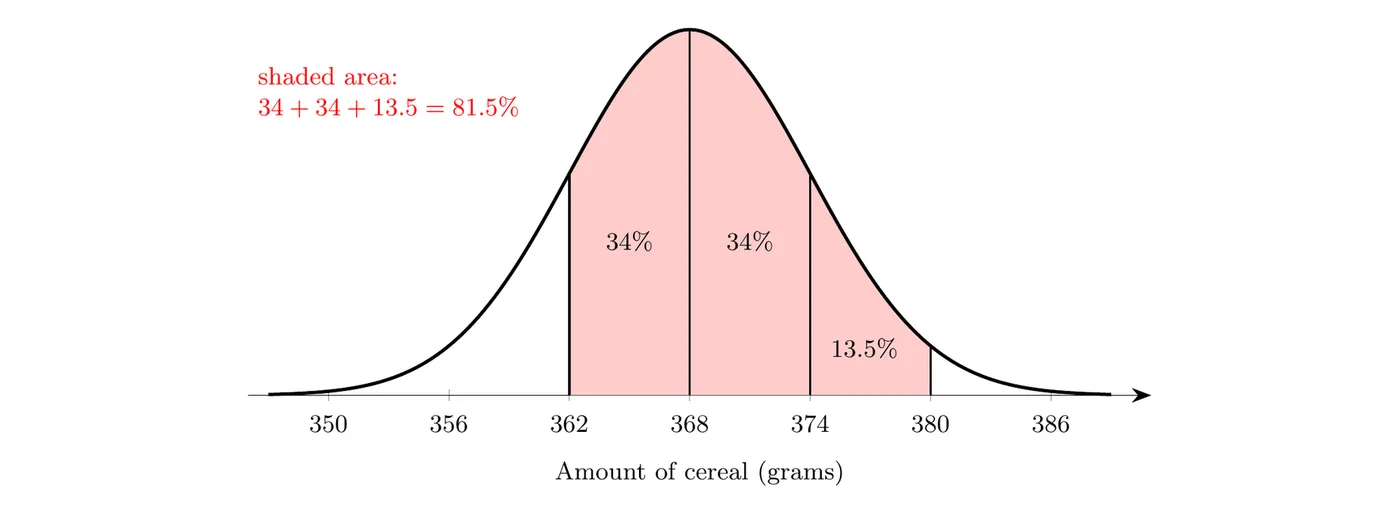
Answer: about 95% of boxes contain between 356 and 380 grams, about 16% contain more than 374 grams, and about 81.5% contain between 362 and 380 grams.

Finding probabilities with a normal distribution

If a random variable is approximately normal, the probability that it falls in an interval is the area under the normal curve over that interval. The total area under the curve is 1. Use these steps:

Name the distribution and the event. Define the variable, say it's normal with its mean and standard deviation, and write the probability you want, like $P(55 < X < 64)$ .

Sketch and shade. Draw the curve, label the mean and the boundary values, and shade the region you want.

Calculate. Either find $z$ -scores and use Table A, or use technology: normalcdf(lower, upper, μ, σ).

Answer in context.

Steps 1 and 2 aren't busywork. On the AP exam, a normal calculation needs the distribution, its parameters, and the boundary and direction of the region. A labeled, shaded sketch shows all of that.

Example 2: Egg weights (AP-style)

Suppose the weights of eggs from a large farm are approximately normal with mean 58 grams (g) and standard deviation 4 g. What is the probability that a randomly selected egg from this farm weighs between 55 g and 64 g?

Step 1: Name the distribution and the event.

X

= the weight of a randomly selected egg, which is approximately normal with

\mu = 58

g and

\sigma = 4

g. We want

P(55 < X < 64)

Step 2: Sketch and shade.

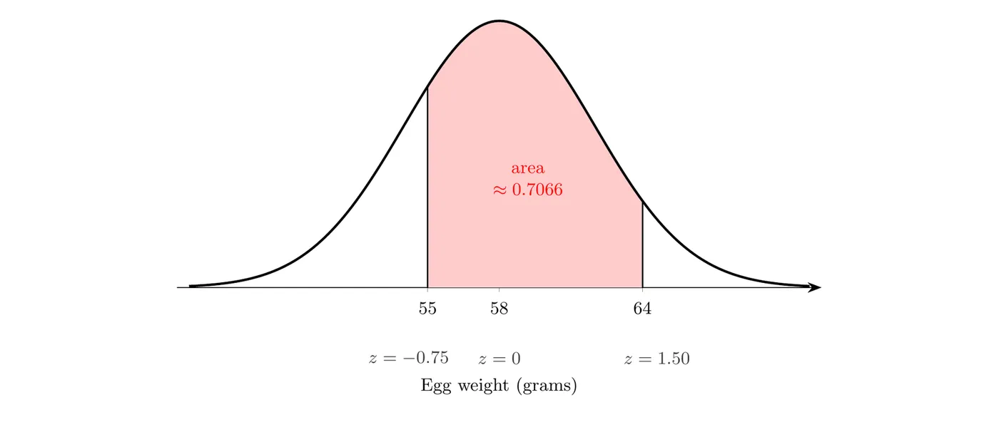
Step 3: Calculate. Find the

z

-scores for the boundaries:

z_1 = \frac{55 - 58}{4} = -0.75 \qquad z_2 = \frac{64 - 58}{4} = 1.50

Table A gives the area to the left of each

z

-score: 0.2266 for

z = -0.75

and 0.9332 for

z = 1.50

. The area between them is the difference:

P(55 < X < 64) \approx 0.9332 - 0.2266 = 0.7066

With technology, normalcdf(55, 64, 58, 4)

\approx 0.7066

Answer: the probability is about 0.707. About 70.7% of eggs from this farm weigh between 55 and 64 grams.

Regions with only one boundary: for

P(X > 64)

, use normalcdf(64, 1E99, 58, 4). For

P(X < 55)

, use

-

1E99 as the lower bound. With Table A, the area to the right of a

z

-score is 1 minus the table value.

Finding values from areas

Sometimes you know an area and need the boundary instead, like "what weight separates the lightest 5% of boxes from the rest?" The boundaries of an interval with a given area can be found two ways:

Technology: invNorm(area, μ, σ) gives the value with that much area to its left. (Newer TI-84s also ask for a tail: LEFT, CENTER, or RIGHT.)

Table A: find the area inside the table, read off the $z$ -score, then convert back to the original units with $x = \mu + z\sigma$ .

Setting up the interval

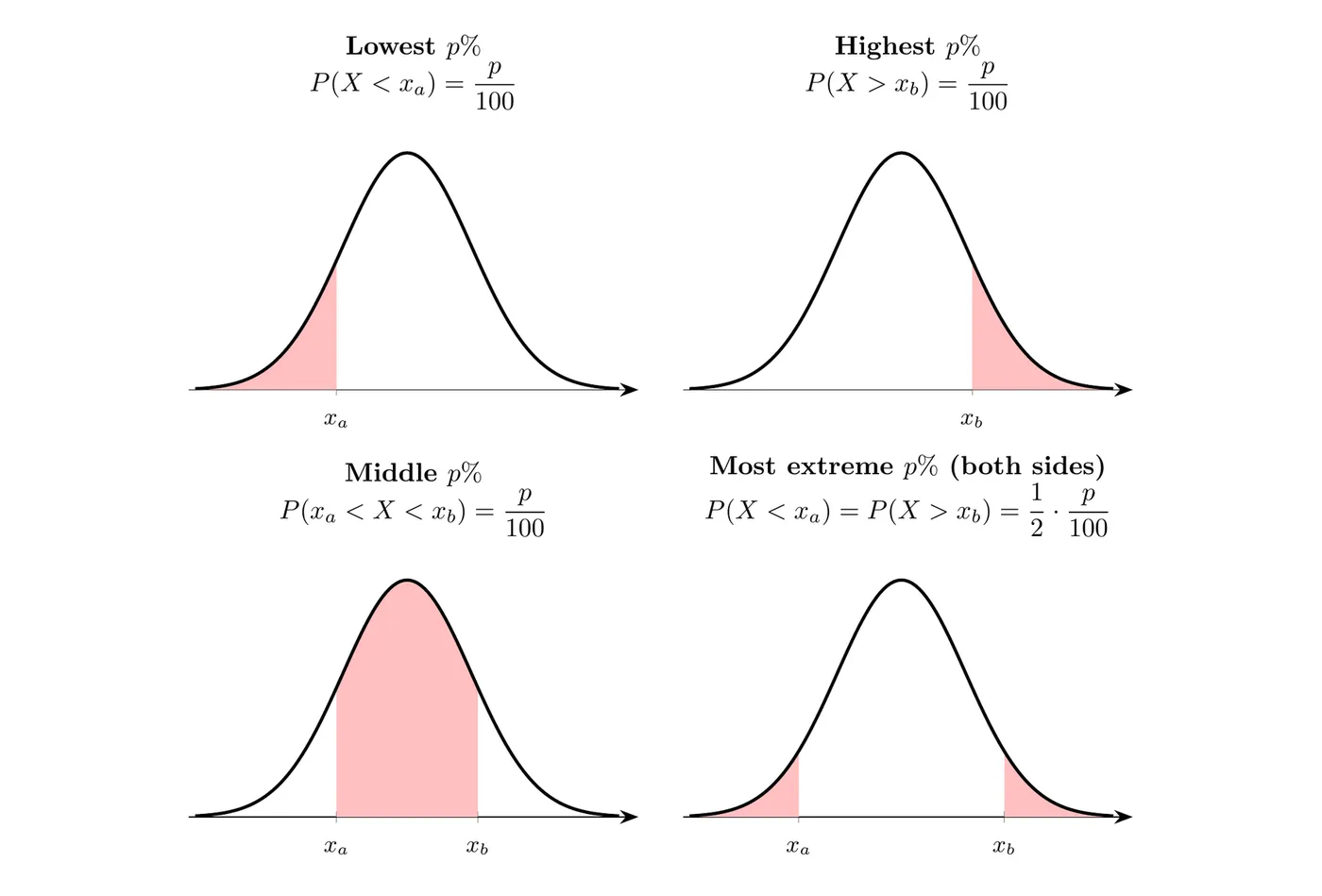
Let

p

be a number between 0 and 100,

x_a

the lower bound, and

x_b

the upper bound. There are four standard setups, and the inequality you write tells you which area to use:

You want	Write	Meaning
the lowest $p\%$	$P(X < x_a) = \frac{p}{100}$	the lowest $p\%$ of values lie to the left of $x_a$
the middle $p\%$	$P(x_a < X < x_b) = \frac{p}{100}$	$p\%$ of values lie between $x_a$ and $x_b$
the highest $p\%$	$P(X > x_b) = \frac{p}{100}$	the highest $p\%$ of values lie to the right of $x_b$
the most extreme $p\%$ on both sides	$P(X < x_a) = \frac{1}{2}\left(\frac{p}{100}\right)$ and $P(X > x_b) = \frac{1}{2}\left(\frac{p}{100}\right)$	half of the extreme $p\%$ lie to the left of $x_a$ and half lie to the right of $x_b$

Since invNorm and Table A both use the area to the left, convert first. For the highest

p\%

, the area to the left of

x_b

1 - \frac{p}{100}

. For the middle

p\%

, the leftover area splits evenly into two tails.

Example 3: Cereal cutoffs

The cereal amounts are approximately normal with

\mu = 368

grams and

\sigma = 6

grams. Find (a) the cutoff for the lightest 5% of boxes, (b) the boundaries of the middle 90%, and (c) the cutoff for the heaviest 10%.

(a) We need

P(X < x_a) = 0.05

. invNorm(0.05, 368, 6)

\approx 358.13

. With Table A, the area 0.05 falls between

z = -1.64

and

z = -1.65

, so

z \approx -1.645

x_a = 368 + (-1.645)(6) \approx 358.13 \text{ grams}

(b) The middle 90% leaves 10% in the tails, 5% on each side. The lower boundary is the 358.13 grams from part (a). The upper boundary has area 0.95 to its left: invNorm(0.95, 368, 6)

\approx 377.87

, which is

368 + 1.645(6)

(c) We need

P(X > x_b) = 0.10

, so the area to the left is 0.90. invNorm(0.90, 368, 6)

\approx 375.69

. With Table A, the closest area to 0.90 is 0.8997 at

z = 1.28

, giving

368 + 1.28(6) = 375.68

Answer: (a) boxes under about 358.1 grams are the lightest 5%. (b) The middle 90% of boxes contain between about 358.1 and 377.9 grams. (c) The heaviest 10% contain more than about 375.7 grams. (For the most extreme

p\%

on both sides, split the area in half the same way: for 4%, use areas 0.02 and 0.98.)

Solving for the mean or standard deviation

If you know one parameter and one percentile, you can solve for the other parameter. Write the

z

-score formula with the known pieces and solve.

Example 4: Adjusting the machine (AP-style)

The cereal boxes are labeled 360 grams. The company wants only 2% of boxes to contain less than 360 grams. (a) If the standard deviation stays at 6 grams, what mean should the machine be set to? (b) If the mean stays at 368 grams, what standard deviation would the machine need?

Step 1: Find the cutoff in standard units. The

z

-score with area 0.02 to its left is invNorm(0.02, 0, 1)

\approx -2.054

. (Table A gives

z \approx -2.05

Step 2 (a): Solve for the mean.

-2.054 = \frac{360 - \mu}{6} \quad \Rightarrow \quad \mu = 360 + 2.054(6) \approx 372.3 \text{ grams}

Step 2 (b): Solve for the standard deviation.

-2.054 = \frac{360 - 368}{\sigma} \quad \Rightarrow \quad \sigma = \frac{-8}{-2.054} \approx 3.9 \text{ grams}

Answer: the company could raise the mean fill to about 372.3 grams, or keep the mean at 368 grams and make the machine more consistent, with a standard deviation of about 3.9 grams. Either way, only 2% of boxes would contain less than the labeled 360 grams.

Comparing relative position with percentiles

Percentiles and proportions can be used to compare the relative positions of values within one normal distribution or between different normal distributions. A value's percentile in a normal distribution is the area to its left, written as a percent. Topic 1.9 compared values from different distributions with

z

-scores. When both distributions are approximately normal, you can go one step further and turn each

z

-score into a percentile.

Example 5: Which score is better?

Suppose scores on Exam A are approximately normal with mean 1050 and standard deviation 200, and scores on Exam B are approximately normal with mean 21 and standard deviation 5. Priya scores 1250 on Exam A. Luis scores 27 on Exam B. Who did better compared with the other people who took the same exam?

Step 1: Standardize each score.

z_{\text{Priya}} = \frac{1250 - 1050}{200} = 1.00 \qquad z_{\text{Luis}} = \frac{27 - 21}{5} = 1.20

Step 2: Find each percentile. Table A gives 0.8413 for

z = 1.00

and 0.8849 for

z = 1.20

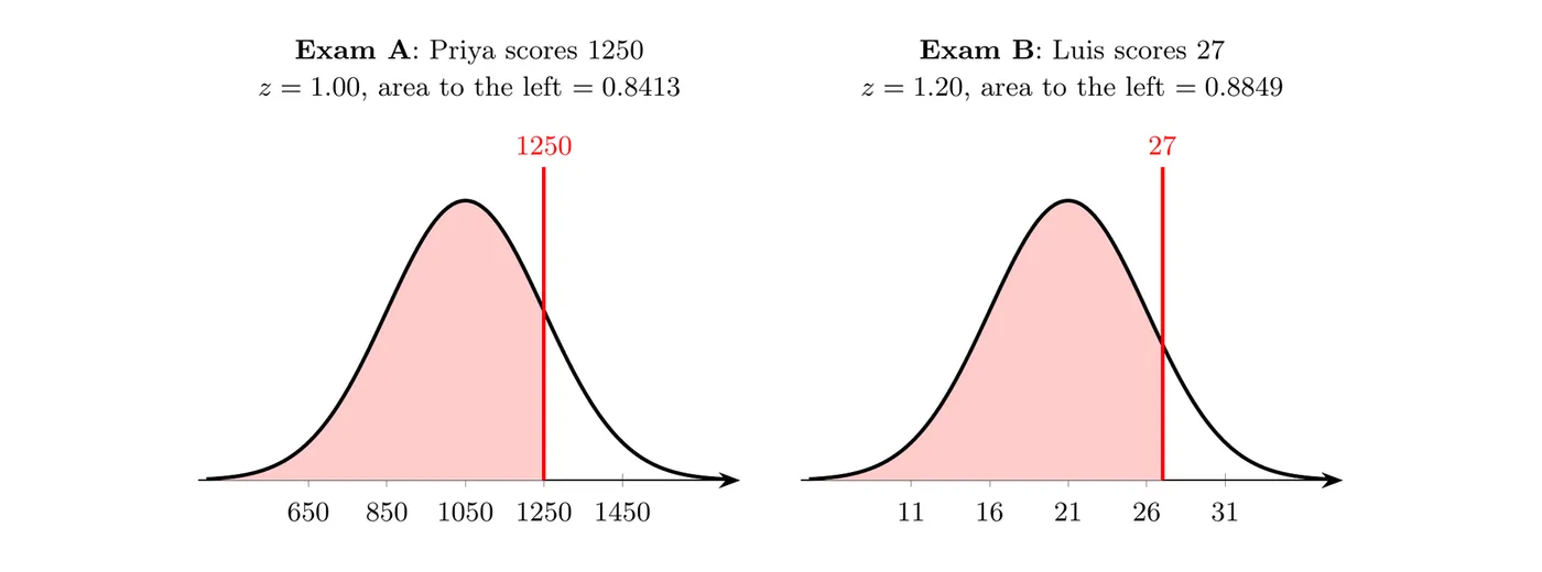
Answer: Priya scored higher than about 84.1% of Exam A test takers, and Luis scored higher than about 88.5% of Exam B test takers. Relative to the people taking the same exam, Luis did better, even though 27 is a much smaller number than 1250.

Common mistakes

Using the empirical rule for boundaries that aren't exactly 1, 2, or 3 standard deviations from the mean. Use normalcdf or Table A instead.

Forgetting that Table A gives the area to the left. For "greater than," subtract the table value from 1.

Mixing up normalcdf and invNorm. normalcdf goes from values to an area. invNorm goes from an area to a value.

Giving invNorm the wrong area. For the heaviest 10%, the area to the left is 0.90, not 0.10.

Writing only calculator syntax. Name the distribution with its mean and standard deviation, and show the boundary and direction. A labeled sketch does both.

Assuming everything is normal. Use normal calculations only when the problem says the distribution is approximately normal or you have good reason to believe it is. For a strongly skewed distribution, the empirical rule and normalcdf give wrong answers.

Back Next