2.8 - Introduction to Random Variables and Probability Distributions

Overview

A random variable turns the results of a random process into numbers, like the number of heads in three coin flips or the number of tacos a customer orders. Its probability distribution lists every possible value and how likely each one is. This topic is about building and reading these distributions as tables, graphs, and formulas, including the cumulative distribution. The rest of the unit builds on it: the mean and standard deviation in Topic 2.9, the binomial distribution in 2.10, and the normal distribution in 2.11.

Random variables

A random variable is a variable whose values are numerical outcomes of a random phenomenon. Each time the random process runs, the random variable takes one value.

Use a capital letter for the random variable, like $X$ , and a lowercase letter for one of its values, like $x$ .

$P(X = 2)$ means "the probability that $X$ takes the value 2."

Example: flip a coin 3 times and let $X$ = the number of heads. The outcome HTH gives $X = 2$ . The possible values of $X$ are 0, 1, 2, and 3.

Discrete and continuous random variables

A discrete random variable has a countable set of possible values, usually counts like 0, 1, 2, 3. You can list them. This topic and topics 2.9 and 2.10 are about discrete random variables.

A continuous random variable can take any value in an interval, like a height or a time. Its probabilities are areas under a curve. The normal distribution in Topic 2.11 is the main example.

Probability distributions

The probability distribution of a discrete random variable gives the probability of every possible value. It's usually written as a table:

Value $x$	$x_1$	$x_2$	$x_3$	$\cdots$
Probability $P(X = x)$	$p_1$	$p_2$	$p_3$	$\cdots$

Every valid probability distribution meets two requirements:

Each probability is between 0 and 1, inclusive.

The probabilities add up to exactly 1: $\sum P(x_i) = 1$ . Every trial produces exactly one value, so all the values together cover the whole sample space.

If either requirement fails, the table is not a valid probability distribution. The second requirement is also how you find a missing probability.

Example 1: Finding a missing probability

A taco truck owner tracks how many tacos each customer orders. Let

X

= the number of tacos ordered by a randomly chosen customer.

$x$	1	2	3	4	5
$P(X = x)$	0.20	0.35	0.25	?	0.05

Find

P(X = 4)

The probabilities must add to 1, so

P(X = 4) = 1 - (0.20 + 0.35 + 0.25 + 0.05) = 1 - 0.85 = 0.15

Answer:

P(X = 4) = 0.15

. About 15% of customers order 4 tacos. (Topic 2.9 uses this same distribution to find the mean number of tacos per customer.)

Building a distribution with probability rules

One way to find a probability distribution is with the rules from topics 2.4 to 2.7: list the outcomes, find the probability of each one, and group the outcomes by the value of the random variable.

Example 2: Number of heads in three flips

Flip a fair coin 3 times and let

X

= the number of heads. Find the probability distribution of

X

Step 1: List the sample space. There are

2 \cdot 2 \cdot 2 = 8

equally likely outcomes: HHH, HHT, HTH, THH, HTT, THT, TTH, TTT.

Step 2: Count the outcomes for each value of

X

. Only TTT has 0 heads. HTT, THT, and TTH have 1 head. HHT, HTH, and THH have 2 heads. Only HHH has 3 heads.

Step 3: Divide each count by 8.

$x$	0	1	2	3
$P(X = x)$	$\frac{1}{8} = 0.125$	$\frac{3}{8} = 0.375$	$\frac{3}{8} = 0.375$	$\frac{1}{8} = 0.125$

Check:

0.125 + 0.375 + 0.375 + 0.125 = 1

. The distribution is symmetric, centered at 1.5 heads.

Example 3: Outcomes that aren't equally likely

A player makes 70% of her free throws, and her shots are independent. She shoots 2 free throws. Let

X

= the number she makes. Find the probability distribution of

X

Step 1:

X = 0

means miss, then miss. The shots are independent, so multiply.

P(X = 0) = 0.3(0.3) = 0.09

Step 2:

X = 1

can happen two ways: make then miss, or miss then make. Each way has probability

0.21

, and the two ways are mutually exclusive, so add them.

P(X = 1) = 0.7(0.3) + 0.3(0.7) = 0.21 + 0.21 = 0.42

Step 3:

X = 2

means make, then make.

P(X = 2) = 0.7(0.7) = 0.49

$x$	0	1	2
$P(X = x)$	0.09	0.42	0.49

Check:

0.09 + 0.42 + 0.49 = 1

. Making both shots is the most likely result, because each shot is more likely to go in than not.

Estimating a distribution with simulation

When the rules get messy, you can estimate a probability distribution with a simulation (Topic 2.3). Run the random process many times, record the value of the random variable each time, and use the relative frequencies as estimates of the probabilities. By the law of large numbers, the estimates get closer to the true probabilities as the number of trials grows.

Example 4: Collecting prizes

A cereal brand puts one of 3 different prizes in each box, and each prize is equally likely. You buy 4 boxes. Let

X

= the number of different prizes you get.

X

can be 1, 2, or 3. Estimate the probability distribution of

X

Step 1: Design the simulation. Label the prizes 1, 2, and 3. For one trial, generate 4 random integers from 1 to 3, one for each box (on a TI-84, randInt(1,3,4)), and record how many different numbers show up. For example, 2, 3, 2, 2 gives

X = 2

Step 2: Run many trials. One simulation of 500 trials gave these results. The last column shows the exact probabilities, found by counting all

3^4 = 81

equally likely ways the 4 boxes can turn out, for comparison.

$x$	Count in 500 trials	Estimated $P(X = x)$	Exact $P(X = x)$
1	17	$\frac{17}{500} = 0.034$	$\frac{3}{81} \approx 0.037$
2	252	$\frac{252}{500} = 0.504$	$\frac{42}{81} \approx 0.519$
3	231	$\frac{231}{500} = 0.462$	$\frac{36}{81} \approx 0.444$

Step 3: Interpret. The simulation estimates that someone who buys 4 boxes gets all 3 prizes about 46.2% of the time. The estimates are close to the exact values, and they would get closer with more trials.

Three ways to show a distribution

A discrete probability distribution can be shown as a table, a graph, or a function (a formula).

Table

A table lists each value with its probability, like the ones above. It's the most common form on the AP exam.

Graph: the probability histogram

A probability histogram puts the values of

X

on the horizontal axis and probability on the vertical axis. Each value gets one bar, centered on the value, with height equal to its probability. Here is the taco distribution from Example 1:

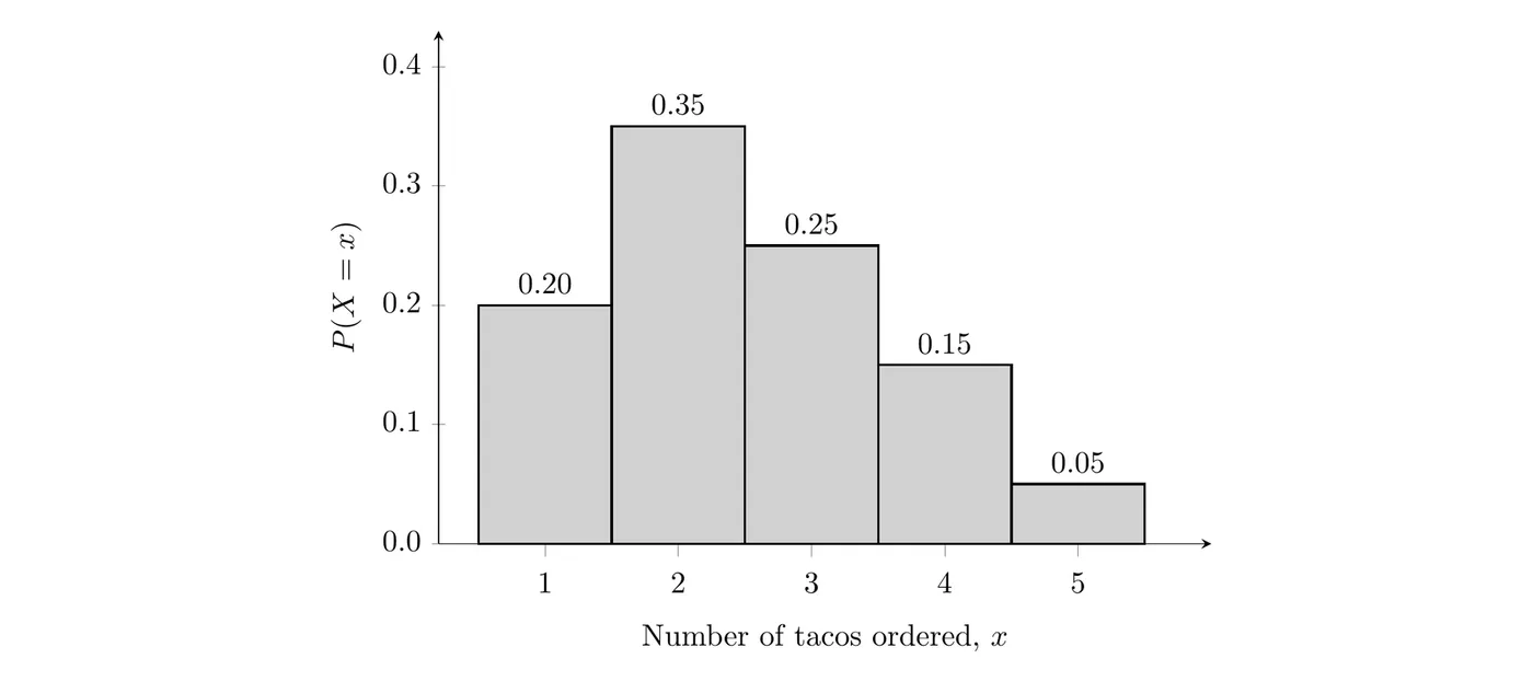
2.8 - Introduction to Random Variables and Probability Distributions

Describe a probability histogram the way you described data distributions in Unit 1. The taco distribution has a single peak at 2 tacos and is skewed right: most customers order 1 to 3 tacos, and fewer order 4 or 5. The bar heights add to 1.

Function

Sometimes the distribution comes as a formula for

P(X = x)

. The binomial formula in Topic 2.10 is the most important example. The same two requirements apply.

Example 5: A distribution given by a formula

A random variable

X

has

P(X = x) = kx

for

x = 1, 2, 3, 4

, where

k

is a constant. Find

k

, then find

P(X = 3)

Step 1: The probabilities must add to 1.

k(1) + k(2) + k(3) + k(4) = 10k = 1 \quad \Rightarrow \quad k = 0.1

Step 2: Use the formula.

P(X = 3) = 0.1(3) = 0.3

Answer:

k = 0.1

, so the probabilities are

0.1

0.2

0.3

, and

0.4

for

x = 1, 2, 3, 4

, and

P(X = 3) = 0.3

Cumulative probability distributions

A cumulative probability distribution gives the probability that

X

is less than or equal to each value,

P(X \le x)

. You build it with running totals: add up the probabilities from the smallest value through

x

. Here is the taco distribution with its cumulative probabilities:

$x$	1	2	3	4	5
$P(X = x)$	0.20	0.35	0.25	0.15	0.05
$P(X \le x)$	0.20	0.55	0.80	0.95	1.00

The cumulative probabilities never go down, and the last one is always 1.

As a function, the cumulative distribution is often written $F(x) = P(X \le x)$ . For example, $F(3) = 0.80$ : 80% of customers order 3 or fewer tacos.

Turning words into inequalities

For a discrete random variable,

<

and

\le

give different answers, so translate the words carefully. For a variable with whole-number values:

Words	Symbols	From the cumulative table
at most 3	$X \le 3$	$P(X \le 3)$
fewer than 3	$X < 3$ , same as $X \le 2$	$P(X \le 2)$
at least 3	$X \ge 3$	$1 - P(X \le 2)$
more than 3	$X > 3$	$1 - P(X \le 3)$
between 2 and 4, inclusive	$2 \le X \le 4$	$P(X \le 4) - P(X \le 1)$

Example 6: Using a cumulative distribution (AP-style)

Use the taco distribution and its cumulative probabilities above. A customer is chosen at random.

(a) Find the probability that the customer orders at most 2 tacos.

P(X \le 2) = 0.20 + 0.35 = 0.55

There's a

0.55

probability that a randomly chosen customer orders 1 or 2 tacos.

(b) Find the probability that the customer orders at least 3 tacos.

P(X \ge 3) = 1 - P(X \le 2) = 1 - 0.55 = 0.45

There's a

0.45

probability that a randomly chosen customer orders 3, 4, or 5 tacos.

(c) Find the probability that the customer orders more than 1 but fewer than 5 tacos. That means

X = 2

3

, or

4

P(2 \le X \le 4) = P(X \le 4) - P(X \le 1) = 0.95 - 0.20 = 0.75

Check by adding the three probabilities:

0.35 + 0.25 + 0.15 = 0.75

. So 75% of customers order 2, 3, or 4 tacos.

(d) The owner claims that most customers order 2 or fewer tacos. Do the probabilities support the claim?

Answer: Yes.

P(X \le 2) = 0.55

, which is greater than

0.5

, so a majority of customers (55%) order 2 or fewer tacos.

Common mistakes

Probabilities that don't add to 1. Always check the sum. If it isn't 1, a value is missing or a probability is wrong.

Treating $<$ and $\le$ as the same. For a discrete variable, $P(X < 3)$ leaves out $X = 3$ , and $P(X \le 3)$ includes it.

Using the wrong complement for "at least." $P(X \ge 3) = 1 - P(X \le 2)$ , not $1 - P(X \le 3)$ .

Confusing an outcome with a value. HTH is an outcome of the random process. $X = 2$ is the value of the random variable for that outcome.

Counts on the vertical axis. A probability histogram shows probabilities, and its bar heights add to 1.

Interpreting without context. Don't stop at $P(X \le 2) = 0.55$ . Say what it means: 55% of customers order 2 or fewer tacos.

Back Next